Conic Sector Goal

Purpose

Enforce sector bound on specific input/output map when using Control System Tuner.

Description

Conic Sector Goal creates a constraint that restricts the output trajectories of a system. If for all nonzero input trajectories u(t), the output trajectory z(t) = (Hu)(t) of a linear system H satisfies:

$\int_{0}^{T} z {(t)}^{T} Q z (t) d t < 0,$

for all T ≥ 0, then the output trajectories of H lie in the conic sector described by the symmetric indefinite matrix Q. Selecting different Q matrices imposes different conditions on the system response. When you create a Conic Sector Goal, you specify the input signals, output signals, and the sector geometry.

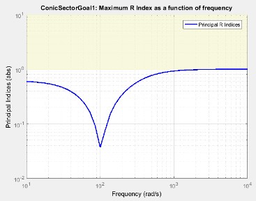
In Control System Tuner, the shaded area on the plot represents the region in the frequency domain in which the tuning goal is not met. The plot shows the value of the R-index described in About Sector Bounds and Sector Indices.

Creation

In the Tuning tab of Control System Tuner, select New Goal > Conic Sector Goal.

Command-Line Equivalent

When tuning control systems at the command line, use TuningGoal.ConicSector to specify a step response goal.

I/O Transfer Selection

Use this section of the dialog box to specify the inputs and outputs of the transfer function that the tuning goal constrains. Also specify any locations at which to open loops for evaluating the tuning goal.

Specify input signals
Select one or more signal locations in your model as inputs to the transfer function that the tuning goal constrains. To constrain a SISO response, select a single-valued input signal. For example, to constrain the gain from a location named 'u' to a location named 'y', click Add signal to list and select 'u'. To constrain the passivity of a MIMO response, select multiple signals or a vector-valued signal.
Specify output signals
Select one or more signal locations in your model as outputs of the transfer function that the tuning goal constrains. To constrain a SISO response, select a single-valued output signal. For example, to constrain the gain from a location named 'u' to a location named 'y', click Add signal to list and select 'y'. To constrain the passivity of a MIMO response, select multiple signals or a vector-valued signal.
Compute input/output gain with the following loops open
Select one or more signal locations in your model at which to open a feedback loop for the purpose of evaluating this tuning goal. The tuning goal is evaluated against the open-loop configuration created by opening feedback loops at the locations you identify. For example, to evaluate the tuning goal with an opening at a location named 'x', click Add signal to list and select 'x'.

Tip

To highlight any selected signal in the Simulink^® model, click . To remove a signal from the input or output list, click . When you have selected multiple signals, you can reorder them using and . For more information on how to specify signal locations for a tuning goal, see Specify Goals for Interactive Tuning.

Options

Specify additional characteristics of the conic sector goal using this section of the dialog box.

Conic Sector Matrix
Enter the sector geometry Q, specified as:
- A matrix, for constant sector geometry. Q is a symmetric square matrix that is ny on a side, where ny is the number of output signals you specify for the goal. The matrix Q must be indefinite to describe a well-defined conic sector. An indefinite matrix has both positive and negative eigenvalues. In particular, Q must have as many negative eigenvalues as there are input signals specified for the tuning goal (the size of the vector input signal u(t)).
- An LTI model, for frequency-dependent sector geometry. Q satisfies Q(s)’ = Q(–s). In other words, Q(s) evaluates to a Hermitian matrix at each frequency.
For more information, see About Sector Bounds and Sector Indices.
Regularization
Regularization parameter, specified as a real nonnegative scalar value. Regularization keeps the evaluation of the tuning goal numerically tractable when other tuning goals tend to make the sector bound ill-conditioned at some frequencies. When this condition occurs, set Regularization to a small (but not negligible) fraction of the typical norm of the feedthrough term in H. For example, if you anticipate the norm of the feedthrough term of H to be of order 1 during tuning, try setting Regularization to 0.001.
For more information about the conditions that require regularization, see the Regularization property of TuningGoal.ConicSector.
Enforce goal in frequency range
Limit the enforcement of the tuning goal to a particular frequency band. Specify the frequency band as a row vector of the form [min,max], expressed in frequency units of your model. For example, to create a tuning goal that applies only between 1 and 100 rad/s, enter [1,100]. By default, the tuning goal applies at all frequencies for continuous time, and up to the Nyquist frequency for discrete time.
Apply goal to
Use this option when tuning multiple models at once, such as an array of models obtained by linearizing a Simulink model at different operating points or block-parameter values. By default, active tuning goals are enforced for all models. To enforce a tuning requirement for a subset of models in an array, select Only Models. Then, enter the array indices of the models for which the goal is enforced. For example, suppose you want to apply the tuning goal to the second, third, and fourth models in a model array. To restrict enforcement of the requirement, enter 2:4 in the Only Models text box.
For more information about tuning for multiple models, see Robust Tuning Approaches (Robust Control Toolbox).

Tips

Constraining Input and Output Trajectories to Conic Sector

Consider the following control system.

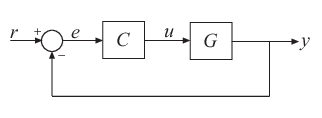
Suppose that the signal u is marked as an analysis point in the model you are tuning. Suppose also that G is the closed-loop transfer function from u to y. A common application is to create a tuning goal that constrains all the I/O trajectories {u(t),y(t)} of G to satisfy:

${\int_{0}^{T} (\begin{matrix} y (t) \\ u (t) \end{matrix})}^{T} Q (\begin{matrix} y (t) \\ u (t) \end{matrix}) d t < 0,$

for all T ≥ 0. Constraining the I/O trajectories of G is equivalent to restricting the output trajectories z(t) of the system H = [G;I] to the sector defined by:

$\int_{0}^{T} z {(t)}^{T} Q z (t) d t < 0.$

(See About Sector Bounds and Sector Indices for more details about this equivalence.) To specify a constraint of this type using Conic Sector Goal, specify u as the input signal, and specify y and u as output signals. When you specify u as both input and output, Conic Sector Goal sets the corresponding transfer function to the identity. Therefore, the transfer function that the goal constrains is H = [G;I] as intended. This treatment is specific to Conic Sector Goal. For other tuning goals, when the same signal appears in both inputs and outputs, the resulting transfer function is zero in the absence of feedback loops, or the complementary sensitivity at that location otherwise. This result occurs because when the software processes analysis points, it assumes that the input is injected after the output. See Mark Signals of Interest for Control System Analysis and Design for more information about how analysis points work.

Algorithms

Let

$Q = W_{1} W_{1}^{T} - W_{2} W_{2}^{T}$

be an indefinite factorization of Q, where $W_{1}^{T} W_{2} = 0$ . If $W_{2}^{T} H (s)$ is square and minimum phase, then the time-domain sector bound

$\int_{0}^{T} z {(t)}^{T} Q z (t) d t < 0,$

is equivalent to the frequency-domain sector condition,

$H (- j ω) Q H (j ω) < 0$

for all frequencies. Conic Sector Goal uses this equivalence to convert the time-domain characterization into a frequency-domain condition that Control System Tuner can handle in the same way it handles gain constraints. To secure this equivalence, Conic Sector Goal also makes $W_{2}^{T} H (s)$ minimum phase by making all its zeros stable. The transmission zeros affected by this minimum-phase condition are the stabilized dynamics for this tuning goal. The Minimum decay rate and Maximum natural frequency tuning options control the lower and upper bounds on these implicitly constrained dynamics. If the optimization fails to meet the default bounds, or if the default bounds conflict with other requirements, on the Tuning tab, use Tuning Options to change the defaults.

For sector bounds, the R-index plays the same role as the peak gain does for gain constraints (see About Sector Bounds and Sector Indices). The condition

$H (- j ω) Q H (j ω) < 0$

is satisfied at all frequencies if and only if the R-index is less than one. The plot that Control System Tuner displays for Conic Sector Goal shows the R-index value as a function of frequency (see sectorplot).

When you tune a control system, the software converts each tuning goal into a normalized scalar value f(x), where x is the vector of free (tunable) parameters in the control system. The software then adjusts the parameter values to minimize f(x) or to drive f(x) below 1 if the tuning goal is a hard constraint.

For Conic Sector Goal, for a closed-loop transfer function H(s,x) from the specified inputs to the specified outputs, f(x) is given by:

$f (x) = \frac{R}{1 + R / R_{\max}}, R_{\max} = 10^{6} .$

R is the relative sector index (see getSectorIndex) of H(s,x), for the sector represented by Q.