About Sector Bounds and Sector Indices
Conic Sectors
In its simplest form, a conic sector is the 2-D region delimited by two lines, and .
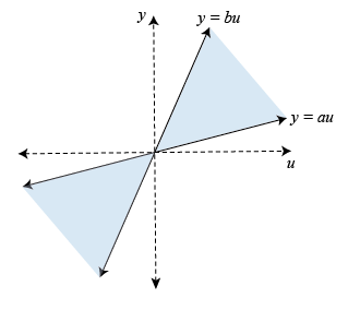
The shaded region is characterized by the inequality . More generally, any such sector can be parameterized as:
where is a 2x2 symmetric indefinite matrix ( has one positive and one negative eigenvalue). We call the sector matrix. This concept generalizes to higher dimensions. In an N-dimensional space, a conic sector is a set:
where is again a symmetric indefinite matrix.
Sector Bounds
Sector bounds are constraints on the behavior of a system. Gain constraints and passivity constraints are special cases of sector bounds. If for all nonzero input trajectories , the output trajectory of a linear system satisfies:
then the output trajectories of lie in the conic sector with matrix . Selecting different matrices imposes different conditions on the system's response. For example, consider trajectories and the following values:
These values correspond to the sector bound:
This sector bound is equivalent to the passivity condition for :
In other words, passivity is a particular sector bound on the system defined by:
Frequency-Domain Condition
Because the time-domain condition must hold for all , deriving an equivalent frequency-domain bound takes a little care and is not always possible. Let the following:
be (any) decomposition of the indefinite matrix into its positive and negative parts. When is square and minimum phase (has no unstable zeros), the time-domain condition:
is equivalent to the frequency-domain condition:
It is therefore enough to check the sector inequality for real frequencies. Using the decomposition of , this is also equivalent to:
Note that is square when has as many negative eigenvalues as input channels in . If this condition is not met, it is no longer enough (in general) to just look at real frequencies. Note also that if is square, then it must be minimum phase for the sector bound to hold.
This frequency-domain characterization is the basis for sectorplot. Specifically, sectorplot plots the singular values of as a function of frequency. The sector bound is satisfied if and only if the largest singular value stays below 1. Moreover, the plot contains useful information about the frequency bands where the sector bound is satisfied or violated, and the degree to which it is satisfied or violated.
For instance, examine the sector plot of a 2-output, 2-input system for a particular sector.
load("sectorExampleSystem.mat","H1")
Q = [-5.12   2.16  -2.04   2.17
      2.16  -1.22  -0.28  -1.11
     -2.04  -0.28  -3.35   0.00
      2.17  -1.11   0.00   0.18];
sectorplot(H1,Q)
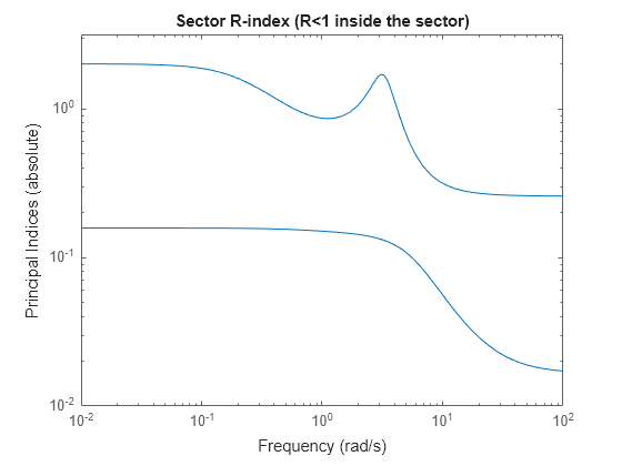
The plot shows that the largest singular value of exceeds 1 below about 0.5 rad/s and in a narrow band around 3 rad/s. Therefore, H does not satisfy the sector bound represented by Q.
Relative Sector Index
We can extend the notion of relative passivity index to arbitrary sectors. Let be an LTI system, and let:
be an orthogonal decomposition of into its positive and negative parts, as is readily obtained from the Schur decomposition of . The relative sector index , or R-index, is defined as the smallest such that for all output trajectories :
Because increasing makes more negative, the inequality is usually satisfied for large enough. However, there are cases when it can never be satisfied, in which case the R-index is . Clearly, the original sector bound is satisfied if and only if .
To understand the geometrical interpretation of the R-index, consider the family of cones with matrix . In 2-D, the cone slant angle is related to by
(see diagram below). More generally, is proportional to . Thus, given a conic sector with matrix , an R-index value means that we can reduce (narrow the cone) by a factor before some output trajectory of leaves the conic sector. Similarly, a value means that we must increase (widen the cone) by a factor to include all output trajectories of . This clearly makes the R-index a relative measure of how well the response of fits in a particular conic sector.
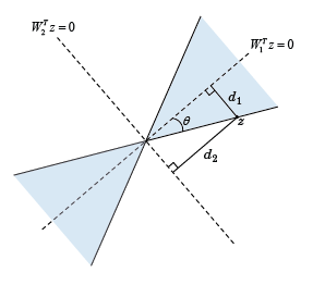
In the diagram,
and
When is square and minimum phase, the R-index can also be characterized in the frequency domain as the smallest such that:
Using elementary algebra, this leads to:
In other words, the R-index is the peak gain of the (stable) transfer function , and the singular values of can be seen as the "principal" R-indices at each frequency. This also explains why plotting the R-index vs. frequency looks like a singular value plot (see sectorplot). There is a complete analogy between relative sector index and system gain. Note, however, that this analogy only holds when is square and minimum phase.
Directional Sector Index
Similarly, we can extend the notion of directional passivity index to arbitrary sectors. Given a conic sector with matrix , and a direction , the directional sector index is the largest such that for all output trajectories :
The directional passivity index for a system corresponds to:
The directional sector index measures by how much we need to deform the sector in the direction to make it fit tightly around the output trajectories of . The sector bound is satisfied if and only if the directional index is positive.
Common Sectors
There are many ways to specify sector bounds. Next we review commonly encountered expressions and give the corresponding system and sector matrix for the standard form used by getSectorIndex and sectorplot:
For simplicity, these descriptions use the notation:
and omit the requirement.
Passivity
Passivity is a sector bound with:
Gain constraint
The gain constraint is a sector bound with:
Ratio of distances
Consider the "interior" constraint,
where are scalars and . This is a sector bound with:
The underlying conic sector is symmetric with respect to . Similarly, the "exterior" constraint,
is a sector bound with:
Double inequality
When dealing with static nonlinearities, it is common to consider conic sectors of the form
where is the nonlinearity output. While this relationship is not a sector bound per se, it clearly implies:
along all I/O trajectories and for all . This condition in turn is equivalent to a sector bound with:
Product form
Generalized sector bounds of the form:
correspond to:
As before, the static sector bound:
implies the integral sector bound above.
QSR dissipative
A system is QSR-dissipative if it satisfies:
This is a sector bound with:
References
[1] Xia, M., P. Gahinet, N. Abroug, C. Buhr, and E. Laroche. “Sector Bounds in Stability Analysis and Control Design.” International Journal of Robust and Nonlinear Control 30, no. 18 (December 2020): 7857–82. https://doi.org/10.1002/rnc.5236.
See Also
getSectorIndex | sectorplot | getSectorCrossover