Tune Control Systems Using systune

Head-Disk Assembly Control

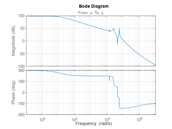
This example uses a 9th-order model of the head-disk assembly (HDA) in a hard-disk drive. This model captures the first few flexible modes in the HDA.

load rctExamples G
bode(G), grid

We use the feedback loop shown below to position the head on the correct track. This control structure consists of a PI controller and a low-pass filter in the return path. The head position y should track a step change r with a response time of about one millisecond, little or no overshoot, and no steady-state error.

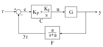
Figure 1: Control Structure

You can use systune to directly tune the PI gains and filter coefficient $$a$$ subject to a variety of time- and frequency-domain requirements.

Specify Tunable Elements

There are two tunable elements in the control structure of Figure 1: the PI controller $$C(s)$$ and the low-pass filter

You can use the tunablePID object to parameterize the PI block:

C0 = tunablePID('C','pi');  % tunable PI

To parameterize the lowpass filter $$F(s)$$, create a tunable real parameter $$a$$ and construct a first-order transfer function with numerator $$a$$ and denominator $$s+a$$:

a = realp('a',1);    % filter coefficient
F0 = tf(a,[1 a]);    % filter parameterized by a

See the "Building Tunable Models" example for an overview of available tunable elements.

Build Tunable Closed-Loop Model

Next build a closed-loop model of the feedback loop in Figure 1. To facilitate open-loop analysis and specify open-loop requirements such as desired stability margins, add an analysis point at the plant input u:

AP = AnalysisPoint('u');

Figure 2: Analysis Point Block

Use feedback to build a model of the closed-loop transfer from reference r to head position y:

T0 = feedback(G*AP*C0,F0);  % closed-loop transfer from r to y
T0.InputName = 'r';
T0.OutputName = 'y';

The result T0 is a generalized state-space model (genss) that depends on the tunable elements $$C$$ and $$F$$.

Specify Design Requirements

To specify the desired behavior of your system, you can define control design requirements using tuning goal objects. You can specify requirements such as the response time, deterministic and stochastic gains, loop shape, stability margins, and pole locations. Here, we use two requirements to capture the control objectives:

Use the TuningGoal.Tracking and TuningGoal.Margins objects to capture these requirements. Note that the margins requirement applies to the open-loop response measured at the plant input u (location marked by the analysis point AP).

Req1 = TuningGoal.Tracking('r','y',0.001);
Req2 = TuningGoal.Margins('u',6,45);

Tune Controller Parameters

You can now use systune to tune the PI gain and filter coefficient $$a$$. This function takes the tunable closed-loop model T0 and the requirements Req1,Req2. Use a few randomized starting points to improve the chances of getting a globally optimal design.

rng('default')
Options = systuneOptions('RandomStart',3);
[T,fSoft] = systune(T0,[Req1,Req2],Options);

Final: Soft = 1.35, Hard = -Inf, Iterations = 72
Final: Soft = 1.35, Hard = -Inf, Iterations = 113
Final: Soft = 2.78e+03, Hard = -Inf, Iterations = 177
       Some closed-loop poles are marginally stable (decay rate near 1e-07)
Final: Soft = 1.35, Hard = -Inf, Iterations = 63

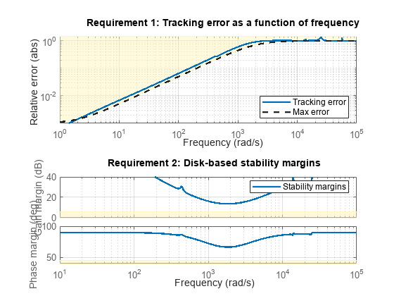
All requirements are normalized so a requirement is satisfied when its value is less than 1. Here the final value is slightly greater than 1, indicating that the requirements are nearly satisfied. Use the output fSoft to see the tuned value of each requirement. Here we see that the first requirement (tracking) is slightly violated while the second requirement (margins) is satisfied.

fSoft

fSoft = 1×2

    1.3461    0.6326

The first output T of systune is the "tuned" closed-loop model. Use showTunable or getBlockValue to access the tuned values of the PI gains and filter coefficient:

getBlockValue(T,'C')  % tuned value of PI controller

ans =
 
             1 
  Kp + Ki * ---
             s 

  with Kp = 0.00104, Ki = 0.0122
 
Name: C
Continuous-time PI controller in parallel form.

showTunable(T)  % tuned values of all tunable elements

C =
 
             1 
  Kp + Ki * ---
             s 

  with Kp = 0.00104, Ki = 0.0122
 
Name: C
Continuous-time PI controller in parallel form.
-----------------------------------
a = 3.19e+03

Validate Results

First use viewGoal to inspect how the tuned system does against each requirement. The first plot shows the tracking error as a function of frequency, and the second plot shows the normalized disk margins as a function of frequency (see diskmargin). See the "Creating Design Requirements" example for details.

clf
viewGoal([Req1 Req2],T)

Next plot the closed-loop step response from reference r to head position y. The response has no overshoot but wobbles a little.

clf, step(T)

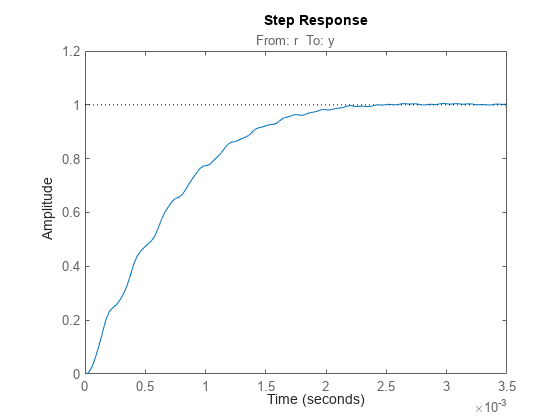
To investigate further, use getLoopTransfer to get the open-loop response at the plant input.

L = getLoopTransfer(T,'u');
bode(L,{1e3,1e6}), grid
title('Open-loop response')

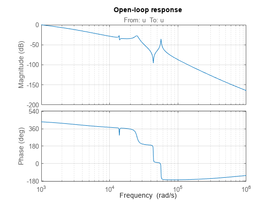
The wobble is due to the first resonance after the gain crossover. To eliminate it, you could add a notch filter to the feedback loop and tune its coefficients along with the lowpass coefficient and PI gains using systune.