Custom Nonlinear ENSO Data Analysis

This example fits the ENSO data using several custom nonlinear equations. The ENSO data consists of monthly averaged atmospheric pressure differences between Easter Island and Darwin, Australia. This difference drives the trade winds in the southern hemisphere.

The ENSO data is clearly periodic, which suggests it can be described by a Fourier series:

$y (x) = a_{0} + \sum_{i = 1}^{\infty} a_{i} \cos (2 π \frac{x}{c_{i}}) + b_{i} \sin (2 π \frac{x}{c_{i}})$

where a_i and b_i are the amplitudes, and c_i are the periods (cycles) of the data. Determine how many cycles exist.

As a first attempt, assume a single cycle and fit the data using one cosine term and one sine term.

$y_{1} (x) = a_{0} + a_{1} \cos (2 π \frac{x}{c_{1}}) + b_{1} \sin (2 π \frac{x}{c_{1}})$

If the fit does not describe the data well, add additional cosine and sine terms with unique period coefficients until a good fit is obtained.

The equation is nonlinear because an unknown coefficient c₁ is included as part of the trigonometric function arguments.

Load Data and Fit Library and Custom Fourier Models

Load the data and open the Curve Fitter app.
```
load enso
curveFitter
```
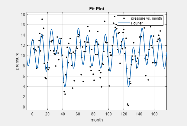
The app includes the Fourier series as a nonlinear library equation. However, the library equation does not meet the needs of this example because its terms are defined as fixed multiples of the fundamental frequency w. Refer to Fit Fourier Models for more information. Create the built-in library Fourier fit to compare with your custom equations:
1. In the app, on the Curve Fitter tab, in the Data section, click Select Data. In the Select Fitting Data dialog box, select month as the X data value and pressure as the Y data value.
2. On the Curve Fitter tab, in the Fit Type section, click the arrow to open the gallery. In the fit gallery, click Fourier in the Regression Models group.
3. In the Table Of Fits pane, double-click the Fit name value and enter Fourier.
4. In the Fit Options pane, change the number of terms to 8.
  Observe the library model fit. In the next steps, you will create custom equations to compare.
Duplicate your fit. Right-click your fit in the Table Of Fits pane and select Duplicate "Fourier".
Name the new fit Enso1Period.
On the Curve Fitter tab, in the Fit Type section, open the fit type gallery and click Custom Equation in the Custom group.
In the Fit Options pane, replace the example text in the equation edit box with the following:
```
a0 + a1*cos(2*pi*x/c1) + b1*sin(2*pi*x/c1)
```
The app applies the fit to the enso data.

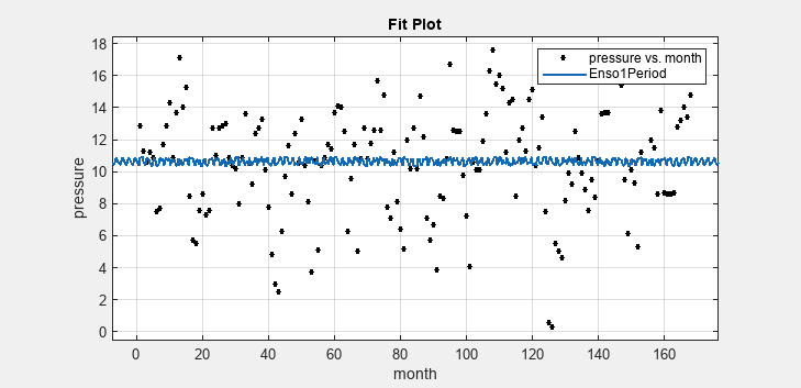
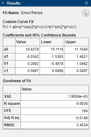
The graphical and numerical results shown here indicate that the fit does not describe the data well. In particular, the fitted value for c1 is unreasonably small. Your initial fit results might differ from these results because the starting points are randomly selected.

Custom equation fit plot for the ENSO data

Results pane for the custom equation fit to the ENSO data

By default, the coefficients are unbounded and have random starting values from 0 to 1. The data include a periodic component with a period of about 12 months. However, with c1 unconstrained and with a random starting point, this fit failed to find that cycle.

Use Fit Options to Constrain a Coefficient

To assist the fitting procedure, constrain c1 to a value from 10 to 14. In the Fit Options pane, click Advanced Options to expand the section and view the constraints for the coefficients. Observe that by default the coefficients are unbounded (bounds of -Inf and Inf).
In the Coefficient Constraints table, change the Lower and Upper bounds for c1 to constrain the cycle from 10 to 14 months, as shown next.
The Curve Fitter app updates the fit.
Observe the new fit and the residuals plot. If necessary, click Residuals Plot in the Visualization section of the Curve Fitter tab.
The fit appears to be reasonable for some data points but clearly does not describe the entire data set very well. As predicted, the numerical results in the Results pane (c1=11.94) indicate a cycle of approximately 12 months. However, the residuals show a systematic periodic distribution, indicating that at least one more cycle exists. There are additional cycles that you should include in the fit equation.

Create Second Custom Fit with Additional Terms and Constraints

To refine your fit, you need to add an additional sine and cosine term to y₁(x) as follows:

$y_{2} (x) = y_{1} (x) + a_{2} \cos (2 π \frac{x}{c_{2}}) + b_{2} \sin (2 π \frac{x}{c_{2}})$

and constrain the upper and lower bounds of c₂ to be roughly twice the bounds used for c₁.

Duplicate your fit by right-clicking it in the Table Of Fits pane and selecting Duplicate "Enso1Period".
Name the new fit Enso2Period.
In the Fit Options pane, add two terms to the end of the previous equation so that the equation box displays the following terms:
```
a0 + a1*cos(2*pi*x/c1) + b1*sin(2*pi*x/c1) + 
a2*cos(2*pi*x/c2) + b2*sin(2*pi*x/c2)
```
Click Advanced Options to expand the section. In the Coefficient Constraints table, observe the Lower and Upper bounds for c1, which constrain the cycle from 10 to 14 months. Add more coefficient constraints.
1. Change the Lower and Upper bounds for c2 to be roughly twice the bounds used for c1 (20<c2<30).
2. Change the StartPoint value for a0 to 5.
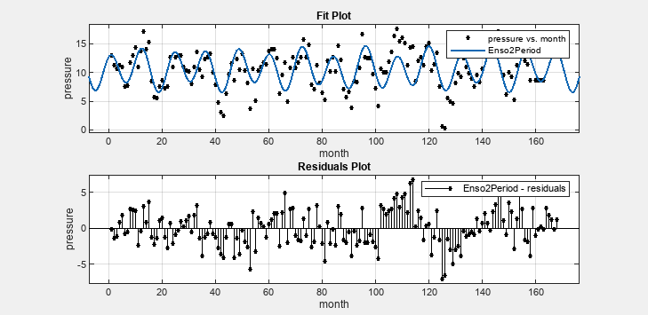
As you change each setting, the Curve Fitter app updates the fit. You can observe the fit plot and the residuals plot.

Fit and residuals plots for the Enso2Period fit

The fit appears reasonable for most data points. However, the residuals indicate that you should include another cycle to the fit equation.

Create a Third Custom Fit with Additional Terms and Constraints

As a third attempt, add an additional sine and cosine term to y₂(x)

$y_{3} (x) = y_{2} (x) + a_{3} \cos (2 π \frac{x}{c_{3}}) + b_{3} \sin (2 π \frac{x}{c_{3}})$

and constrain the lower bound of c₃ to be roughly triple the value of c₁.

Duplicate your fit by right-clicking it in the Table Of Fits pane and selecting Duplicate "Enso2Period".
Name the new fit Enso3Period.
In the Fit Options pane, add two terms to the end of the previous equation so that the equation box displays the following terms:
```
a0 + a1*cos(2*pi*x/c1) + b1*sin(2*pi*x/c1) + 
a2*cos(2*pi*x/c2) + b2*sin(2*pi*x/c2) +
a3*cos(2*pi*x/c3) + b3*sin(2*pi*x/c3)
```
Click Advanced Options to expand the section. Observe that your previous fit options are still present.
In the Coefficient Constraints table, change the Lower bound for c3 to 36, which is roughly triple the value of c1.
As you change each setting, the Curve Fitter app updates the fit. You can observe the fit plot and the residuals plot.

Fit and residuals plots for the Enso3Period fit

The fit is an improvement over the previous two fits, and appears to account for most of the cycles in the ENSO data set. The residuals appear random for most of the data, although a pattern is still visible indicating that additional cycles might be present, or you can improve the fitted amplitudes.

In conclusion, Fourier analysis of the data reveals three significant cycles. The annual cycle is the strongest, but cycles with periods of approximately 44 and 22 months are also present. These cycles correspond to El Nino and the Southern Oscillation (ENSO).