Fit Fourier Models

About Fourier Series Models

A Fourier series describes a periodic function as a sum of sine and cosine functions. You can separate an arbitrary periodic function into simple components by using a Fourier series. These components are easy to integrate, differentiate, and analyze. For this reason, Fourier series are often used to approximate periodic signals.

Fourier series are represented in several forms. Curve Fitting Toolbox™ uses the trigonometric Fourier series form

$y = a_{0} + \sum_{i = 1}^{n} a_{i} \cos (i w x) + b_{i} \sin (i w x)$

where a₀ models a constant (intercept) term in the data and is associated with the i = 0 cosine term, w is the fundamental frequency of the signal, and n is the number of terms (harmonics). Curve Fitting Toolbox supports Fourier series regression for 1 ≤ n ≤ 8.

For more information about Fourier series, refer to Fourier Analysis and Filtering.

Fit Fourier Model Interactively in Curve Fitter App

Open Live Script

This example shows how to use the Curve Fitter app to fit a Fourier model to data.

Load the sound signal sample data.

load gong.mat

The variables y and Fs contain sound signal and frequency data for a gong ring, respectively. Create a sound clip by storing the first 1000 elements of y in a vector named gongClip.

gongClip = y(1:1000);

To calculate the time corresponding to each element in gongClip, divide the index of the elements by Fs.

t = [1:1000]./Fs;

Open the Curve Fitter app from the command line.

curveFitter

Alternatively, on the Apps tab, in the Math, Statistics and Optimization group, click Curve Fitter.

In the Curve Fitter app, select the data variables for the fit. On the Curve Fitter tab, in the Data section, click Select Data. In the Select Fitting Data dialog box, select t as the X data value and gongClip as the Y data value.

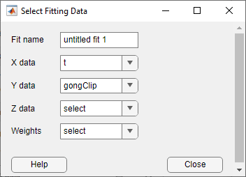
The app plots the data points as you select variables. By default, the app fits a polynomial to the data. To fit a Fourier model, click Fourier in the Fit Type section of the Curve Fitter tab.

The app fits a single-term Fourier model.

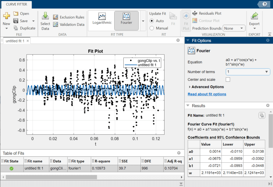
The fitted one-term Fourier model is a periodic function with a simple oscillatory behavior. The Results panel displays the general equation for the model, fitted coefficient estimates with 95% confidence intervals, fundamental frequency, and goodness-of-fit statistics.

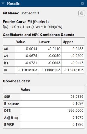
The fitted one-term Fourier model has a root mean square error (RMSE) of 0.1996. To compare the one-term Fourier model with a Fourier model that has four terms, select 4 for Number of terms in the Fit Options panel. The app fits a Fourier model with four terms to the data.

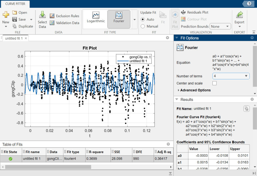
The fitted four-term Fourier model has more complex oscillatory behavior than the one-term Fourier model. An RMSE of 0.1685 for the four-term model indicates that four terms predict the sound data more accurately than one. However, the plot shows that some of the data points in gongClip are outside of the range of the four-term model.

Export the fitted four-term Fourier model to the workspace by clicking Export in the Export section and then selecting Export to Workspace. In the dialog box, uncheck the second and third options. Store the fit in the variable name in the box next to the first option.

You can listen to the sound data in gongClip by using the function sound.

sound(gongClip,Fs)
pause(2)    % Allow gongClip to play before executing next line

To get the sound data for the Fourier model approximation of gongClip, use feval to evaluate gongFourierModel at the times in t. Play the approximated sound data.

gongClipApprox = feval(gongFourierModel,t);
sound(gongClipApprox,Fs)

The two clips have the same approximate average tone. However, the approximated sound data does not have as many fluctuations in tone as the sound data in gongClip.

Fit Fourier Model at the Command Line

Open Live Script

This example shows how to fit a Fourier model to data using the fit function.

Fit Two-Term Fourier Model

Load the El Niño-Southern Oscillation (ENSO) data.

load enso

The variable pressure contains data for the averaged atmospheric pressure difference between Easter Island, Chile and Darwin, Australia. The variable month contains data for the month in which each pressure difference occurred.

Plot pressure against month.

plot(month,pressure)

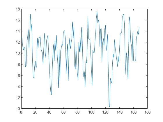
Figure contains an axes object. The axes object contains an object of type line.

The pressure data oscillates between 0 and 18, which indicates that it can be described by a Fourier series.

Fit a two-term Fourier model by using the Fourier library model. Specify the model type as fourier followed by the number of terms. Save the goodness-of-fit statistics for later comparison.

[f2,gof2] = fit(month,pressure,"fourier2")

f2 = 
     General model Fourier2:
     f2(x) =  a0 + a1*cos(x*w) + b1*sin(x*w) + 
               a2*cos(2*x*w) + b2*sin(2*x*w)
     Coefficients (with 95% confidence bounds):
       a0 =       10.63  (10.23, 11.03)
       a1 =       2.923  (2.27, 3.576)
       b1 =       1.059  (0.01593, 2.101)
       a2 =     -0.5052  (-1.086, 0.07532)
       b2 =      0.2187  (-0.4202, 0.8576)
       w =      0.5258  (0.5222, 0.5294)

gof2 = struct with fields:
           sse: 1.1230e+03
       rsquare: 0.4279
           dfe: 162
    adjrsquare: 0.4103
          rmse: 2.6329

f2 is a cfit object containing the general formula, coefficient estimates with 95% confidence bounds, and fundamental frequency for the fit w. The confidence bounds on a2 and b2 cross zero, so not enough evidence exists to conclude that they differ from zero or that the fitted model differs from a one-term Fourier model. The root mean square error (RMSE) of 2.6329 is useful for comparing the accuracy of f2 to the accuracy of other fits.

To calculate the period from the fundamental frequency, use the formula T = 2*pi/w.

w = f2.w

w = 
0.5258

T = 2*pi/w

T = 
11.9497

The period of the fitted two-term Fourier model is approximately 12 months, or one year.

Plot f2 with a scatter plot of the data.

plot(f2,month,pressure)

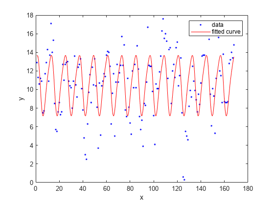
Figure contains an axes object. The axes object with xlabel x, ylabel y contains 2 objects of type line. One or more of the lines displays its values using only markers These objects represent Data, Fitted curve.

The shape of f2 is similar to the shape of a one-term Fourier model, and the oscillation peaks approximately once every 12 months.

Fit Seven-Term Fourier Model

Fit a seven-term Fourier model to the data. Save the goodness-of-fit statistics.

[f7,gof7] = fit(month,pressure,"fourier7")

f7 = 
     General model Fourier7:
     f7(x) = 
               a0 + a1*cos(x*w) + b1*sin(x*w) + 
               a2*cos(2*x*w) + b2*sin(2*x*w) + a3*cos(3*x*w) + b3*sin(3*x*w) + 
               a4*cos(4*x*w) + b4*sin(4*x*w) + a5*cos(5*x*w) + b5*sin(5*x*w) + 
               a6*cos(6*x*w) + b6*sin(6*x*w) + a7*cos(7*x*w) + b7*sin(7*x*w)
     Coefficients (with 95% confidence bounds):
       a0 =       10.63  (10.28, 10.97)
       a1 =      0.5669  (0.08285, 1.051)
       b1 =      0.1969  (-0.29, 0.6838)
       a2 =      -1.203  (-1.687, -0.7189)
       b2 =     -0.8085  (-1.307, -0.31)
       a3 =      0.9323  (0.4325, 1.432)
       b3 =      0.7599  (0.2622, 1.258)
       a4 =     -0.6653  (-1.149, -0.1817)
       b4 =     -0.2038  (-0.6995, 0.292)
       a5 =    -0.02913  (-0.5129, 0.4547)
       b5 =     -0.3701  (-0.8566, 0.1164)
       a6 =    -0.04841  (-0.5437, 0.4469)
       b6 =     -0.1367  (-0.6286, 0.3552)
       a7 =       2.812  (2.19, 3.433)
       b7 =       1.333  (0.4017, 2.264)
       w =     0.07527  (0.07478, 0.07576)

gof7 = struct with fields:
           sse: 768.3656
       rsquare: 0.6086
           dfe: 152
    adjrsquare: 0.5700
          rmse: 2.2483

f7 contains several coefficients with confidence bounds that cross zero, so not enough evidence exists to conclude that their corresponding terms increase the accuracy of the fitted Fourier model. The RMSE of 2.2483 is smaller than the RMSE error of f2, which confirms that the seven-term Fourier model predicts the pressure more accurately than the two-term Fourier model.

To calculate the period from the fundamental frequency, use the formula T = 2*pi/w to calculate the period.

w = f7.w

w = 
0.0753

T = (2*pi)/w

T = 
83.4745

The period of the fitted seven-term Fourier model is approximately 83 months, or roughly seven years. The amplitude of the fitted coefficients determines which terms contribute most to the predicted value of the pressure difference.

The period of a sinusoid of the form sin(Ax) or cos(Ax) is given by the formula T = 2*pi/|A|. a7 and b7 are the largest coefficients.

T = 2*pi/(w*7)

T = 
11.9249

The period of the terms corresponding to a7 and b7 is approximately 12 months, indicating that the annual cycle is the strongest.

Use the same formula to calculate the periods of the following terms:

The terms a1 and b1 have a period of 7 years each.
The terms a2 and b2 have a period of 3.5 (7/2) years each. The a2 and b2 coefficients have larger magnitude than a1 and b1, so the 3.5-year cycle contributes more to the predicted value of the pressure difference than the 7-year cycle.
The terms a3 and b3 are strong, indicating 2.3-year (7/3) cycle.

Smaller terms such as a6, b6, a5, and b5 are less important for the fit.

Plot f7 with a scatter plot of the data.

plot(f7,month,pressure)

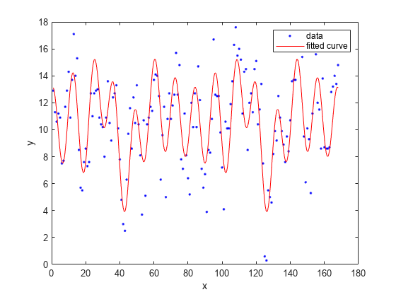
The seven-term Fourier model oscillates in a more complex pattern and captures a wider range of values in the pressure difference than the one-term Fourier model. The cycle repeats approximately every 84 months, or 7 years. Typically, the El Niño warming happens at irregular intervals of two to seven years, and lasts nine months to two years. The average period length is five years. The model results reflect some of these periods.

Set Start Points

The fit function uses the data input argument to calculate optimized start points for the coefficient and fundamental frequency calculations. Fourier series models are particularly sensitive to start points, and the optimized values might be accurate for only a few terms in the associated equations. You can override the optimized start points by specifying the StartPoint name-value argument.

The extreme values in the scatter plot of the data suggest that a four-year cycle might be present. To confirm this suggestion, set the start point of the fundamental frequency to the value corresponding to a period of eight years, or 96 months. An eight-year period for the fitted Fourier model increases the period of the terms a2 and b2 from 3.5 to 4.

w_8 = (2*pi)/96

w_8 = 
0.0654

Find the index of the fundamental frequency in the cell vector of f7 coefficient names by using the coeffnames function.

coeffnames(f7)

ans = 16x1 cell
    {'a0'}
    {'a1'}
    {'b1'}
    {'a2'}
    {'b2'}
    {'a3'}
    {'b3'}
    {'a4'}
    {'b4'}
    {'a5'}
    {'b5'}
    {'a6'}
    {'b6'}
    {'a7'}
    {'b7'}
    {'w' }

The fundamental frequency is in the last entry of the vector of coefficient names. Create a vector of coefficient values from the coefficients of f7, and replace the value for the fundamental frequency with the value corresponding to an eight-year period.

coeffs = coeffvalues(f7);
coeffs(:,end) = w_8

coeffs = 1×16

   10.6262    0.5669    0.1969   -1.2031   -0.8085    0.9323    0.7599   -0.6653   -0.2038   -0.0291   -0.3701   -0.0484   -0.1367    2.8120    1.3330    0.0654

Fit a seven-term Fourier model to the pressure difference data using the coefficients with the new value for the fundamental frequency as the start point. Save the goodness-of-fit statistics.

[f7_8,gof7_8] = fit(month,pressure,"fourier7",StartPoint=coeffs)

f7_8 = 
     General model Fourier7:
     f7_8(x) = 
               a0 + a1*cos(x*w) + b1*sin(x*w) + 
               a2*cos(2*x*w) + b2*sin(2*x*w) + a3*cos(3*x*w) + b3*sin(3*x*w) + 
               a4*cos(4*x*w) + b4*sin(4*x*w) + a5*cos(5*x*w) + b5*sin(5*x*w) + 
               a6*cos(6*x*w) + b6*sin(6*x*w) + a7*cos(7*x*w) + b7*sin(7*x*w)
     Coefficients (with 95% confidence bounds):
       a0 =       10.58  (10.05, 11.1)
       a1 =      0.3286  (-0.4339, 1.091)
       b1 =    -0.05917  (-0.7884, 0.6701)
       a2 =     -0.8667  (-1.738, 0.004258)
       b2 =       1.094  (0.2819, 1.906)
       a3 =     -0.4524  (-1.232, 0.3272)
       b3 =     -0.3117  (-1.099, 0.4753)
       a4 =       0.181  (-0.7949, 1.157)
       b4 =      0.5806  (-0.1796, 1.341)
       a5 =     0.03263  (-0.7174, 0.7827)
       b5 =     -0.2299  (-0.9767, 0.5169)
       a6 =      0.3726  (-0.39, 1.135)
       b6 =     -0.2745  (-1.165, 0.6161)
       a7 =      0.4309  (-0.491, 1.353)
       b7 =     -0.3547  (-1.316, 0.6062)
       w =     0.06795  (0.06519, 0.0707)

gof7_8 = struct with fields:
           sse: 1.6851e+03
       rsquare: 0.1416
           dfe: 152
    adjrsquare: 0.0568
          rmse: 3.3296

The coefficients of f7_8 are slightly shifted from the f7 coefficients. The higher RMSE for f7_8 indicates that f7 is a better fit for the data. Plot both fits to visually compare the models.

plot(f7_8,month,pressure)
hold on
plot(f7, 'b')
hold off
legend("Data","f7_8","f7")

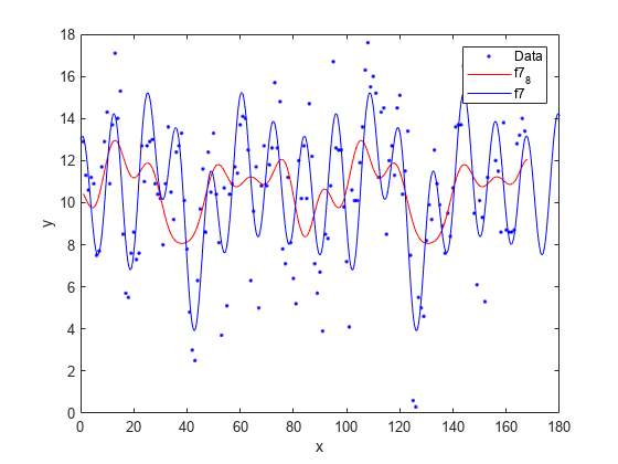
Figure contains an axes object. The axes object with xlabel x, ylabel y contains 3 objects of type line. One or more of the lines displays its values using only markers These objects represent Data, f7_8, f7.

The plot shows that f7 captures the variation in the pressure difference data more accurately than f7_8.

Display Fourier Fit Iterations

An alternative to specifying additional options using name-value arguments is to pass a fitoptions object to the fit function. To view the available options for a Fourier model fit, pass the model name as an input argument to the fitoptions function.

fitoptions("fourier7")

ans = 
  nlsqoptions with properties:

       StartPoint: []
            Lower: []
            Upper: []
        Algorithm: 'Trust-Region'
    DiffMinChange: 1.0000e-08
    DiffMaxChange: 0.1000
          Display: 'Notify'
      MaxFunEvals: 600
          MaxIter: 400
           TolFun: 1.0000e-06
             TolX: 1.0000e-06
           Robust: 'Off'
        Normalize: 'off'
          Exclude: []
          Weights: []
           Method: 'NonlinearLeastSquares'

Create a fitoptions object, and specify to display the output after each iteration.

optionsf7 = fitoptions("fourier7",Display="iter")

optionsf7 = 
  nlsqoptions with properties:

       StartPoint: []
            Lower: []
            Upper: []
        Algorithm: 'Trust-Region'
    DiffMinChange: 1.0000e-08
    DiffMaxChange: 0.1000
          Display: 'Iter'
      MaxFunEvals: 600
          MaxIter: 400
           TolFun: 1.0000e-06
             TolX: 1.0000e-06
           Robust: 'Off'
        Normalize: 'off'
          Exclude: []
          Weights: []
           Method: 'NonlinearLeastSquares'

optionsf7 is a fitoptions object that contains the options for a seven-term Fourier model fit.

To view the iteration steps involved in creating f7, fit another seven-term Fourier model using the options in optionsf7.

f7_iter = fit(month,pressure,"fourier7",optionsf7)

                                         Norm of      First-order 
 Iteration  Func-count     f(x)          step          optimality   CG-iterations
     0          2          768.41                      1.93e+03
     1          4         768.366     2.2176e-05           69.1            0
     2          6         768.366    7.94962e-07           2.48            0
Success, but fitting stopped because change in residuals less than tolerance (TolFun).

f7_iter = 
     General model Fourier7:
     f7_iter(x) = 
               a0 + a1*cos(x*w) + b1*sin(x*w) + 
               a2*cos(2*x*w) + b2*sin(2*x*w) + a3*cos(3*x*w) + b3*sin(3*x*w) + 
               a4*cos(4*x*w) + b4*sin(4*x*w) + a5*cos(5*x*w) + b5*sin(5*x*w) + 
               a6*cos(6*x*w) + b6*sin(6*x*w) + a7*cos(7*x*w) + b7*sin(7*x*w)
     Coefficients (with 95% confidence bounds):
       a0 =       10.63  (10.28, 10.97)
       a1 =      0.5669  (0.08285, 1.051)
       b1 =      0.1969  (-0.29, 0.6838)
       a2 =      -1.203  (-1.687, -0.7189)
       b2 =     -0.8085  (-1.307, -0.31)
       a3 =      0.9323  (0.4325, 1.432)
       b3 =      0.7599  (0.2622, 1.258)
       a4 =     -0.6653  (-1.149, -0.1817)
       b4 =     -0.2038  (-0.6995, 0.292)
       a5 =    -0.02913  (-0.5129, 0.4547)
       b5 =     -0.3701  (-0.8566, 0.1164)
       a6 =    -0.04841  (-0.5437, 0.4469)
       b6 =     -0.1367  (-0.6286, 0.3552)
       a7 =       2.812  (2.19, 3.433)
       b7 =       1.333  (0.4017, 2.264)
       w =     0.07527  (0.07478, 0.07576)

To investigate the Fourier model fit further, you can experiment with specifying different options available for the NonlinearLeastSquares fitting algorithm. See fitoptions for more information.