如果 Method 一致，则 options2 中属性的非空值将覆盖 newOptions 中 options1 中的对应值。
如果 Method 不同，则 newOptions 包含 Method 的 options1 值，以及来自 Normalize、Exclude 和 Weights 的 options2 的值。

示例

全部折叠

修改默认拟合选项以归一化数据

打开实时脚本

创建默认拟合选项对象，并在拟合前将选项设置为中心化并缩放数据。

options = fitoptions;
options.Normal = 'on'

options = 
  basefitoptions with properties:

    Normalize: 'on'
      Exclude: []
      Weights: []
       Method: 'None'

为高斯拟合创建默认拟合选项

打开实时脚本

options = fitoptions('gauss2')

options = 
  nlsqoptions with properties:

          StartPoint: []
           Algorithm: 'Trust-Region'
       DiffMinChange: 1.0000e-08
       DiffMaxChange: 0.1000
             Display: 'Notify'
         MaxFunEvals: 600
             MaxIter: 400
              TolFun: 1.0000e-06
                TolX: 1.0000e-06
               Lower: [-Inf -Inf 0 -Inf -Inf 0]
               Upper: []
    ConstraintPoints: []
              TolCon: 1.0000e-06
              Robust: 'Off'
           Normalize: 'off'
             Exclude: []
             Weights: []
              Method: 'NonlinearLeastSquares'

设置多项式拟合选项

打开实时脚本

为三次多项式创建拟合选项，并设置中心化并缩放以及稳健拟合选项。

options = fitoptions('poly3', 'Normalize', 'on', 'Robust', 'Bisquare')

options = 
  llsqoptions with properties:

               Lower: []
               Upper: []
    ConstraintPoints: []
              TolCon: 1.0000e-06
              Robust: 'Bisquare'
           Normalize: 'on'
             Exclude: []
             Weights: []
              Method: 'LinearLeastSquares'

为线性最小二乘创建拟合选项

打开实时脚本

options = fitoptions('Method', 'LinearLeastSquares')

options = 
  llsqoptions with properties:

               Lower: []
               Upper: []
    ConstraintPoints: []
              TolCon: 1.0000e-06
              Robust: 'Off'
           Normalize: 'off'
             Exclude: []
             Weights: []
              Method: 'LinearLeastSquares'

指定插值拟合的外插方法

打开实时脚本

使用最近邻外插方法为线性插值拟合创建一个 fitoptions 对象。

linearoptions = fitoptions("linearinterp",ExtrapolationMethod="nearest")

linearoptions = 
  linearinterpoptions with properties:

    ExtrapolationMethod: 'nearest'
              Normalize: 'off'
                Exclude: []
                Weights: []
                 Method: 'LinearInterpolant'

使用最近邻外插方法为三次插值拟合创建第二个 fitoptions 对象。

cubicoptions = fitoptions("cubicinterp",ExtrapolationMethod="nearest")

cubicoptions = 
  cubicsplineinterpoptions with properties:

    ExtrapolationMethod: 'nearest'
              Normalize: 'off'
                Exclude: []
                Weights: []
                 Method: 'CubicSplineInterpolant'

您可以使用 linearoptions 中的拟合选项，通过 fit 函数创建一个 linearinterp 拟合对象。使用 cubicoptions 创建一个 cubicinterp 拟合。

在多个拟合中使用相同的拟合选项

打开实时脚本

如果您要设置 Normalize、Exclude 或 Weights 属性，然后使用相同的选项和不同拟合方法对数据进行拟合，则修改默认拟合选项对象结构体非常有用。例如，下面使用相同的拟合选项进行不同的库模型类型拟合。

load census
options = fitoptions;
options.Normalize = 'on';
f1 = fit(cdate,pop,'poly3',options);
f2 = fit(cdate,pop,'exp1',options);
f3 = fit(cdate,pop,'cubicspline',options)

f3 = 
     Cubic interpolating spline:
       f3(x) = piecewise polynomial computed from p
       with cubic extrapolation
       where x is normalized by mean 1890 and std 62.05
     Coefficients:
       p = coefficient structure

查找并更改平滑拟合选项

打开实时脚本

找出平滑参数。数据相关的拟合选项（如 smooth 参量）在 fit 函数的第三个输出参量中返回。

load census
[f,gof,out] = fit(cdate,pop,'SmoothingSpline');
smoothparam = out.p

smoothparam = 
0.0089

修改新拟合的默认平滑参数。

options = fitoptions('Method','SmoothingSpline',...
                     'SmoothingParam',0.0098);
[f,gof,out] = fit(cdate,pop,'SmoothingSpline',options);

应用系数边界来改进高斯拟合

打开实时脚本

创建一个高斯拟合，检查置信区间，并指定下界拟合选项以帮助算法运行。

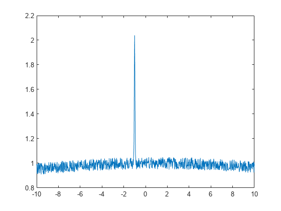
创建两个高斯峰值的含噪总和，其中一个峰的宽度较小，另一个宽度较大。

a1 = 1; b1 = -1; c1 = 0.05;
a2 = 1; b2 = 1; c2 = 50;
x = (-10:0.02:10)';
gdata = a1*exp(-((x-b1)/c1).^2) + ...
        a2*exp(-((x-b2)/c2).^2) + ...
        0.1*(rand(size(x))-.5);
plot(x,gdata)

Figure contains an axes object. The axes object contains an object of type line.

使用双项高斯库模型拟合数据。

gfit = fit(x,gdata,'gauss2')

gfit = 
     General model Gauss2:
     gfit(x) =  a1*exp(-((x-b1)/c1)^2) + a2*exp(-((x-b2)/c2)^2)
     Coefficients (with 95% confidence bounds):
       a1 =     -0.1451  (-1.485, 1.195)
       b1 =       9.725  (-14.7, 34.15)
       c1 =       7.117  (-15.84, 30.07)
       a2 =       14.08  (-1.962e+04, 1.965e+04)
       b2 =       607.4  (-3.197e+05, 3.209e+05)
       c2 =         376  (-9.745e+04, 9.82e+04)

plot(gfit,x,gdata)

Figure contains an axes object. The axes object with xlabel x, ylabel y contains 2 objects of type line. One or more of the lines displays its values using only markers These objects represent Data, Fitted curve.

该算法存在困难，这表现在几个系数的置信区间很宽。

为了帮助算法运行，可指定非负振幅 a1 和 a2 以及宽度 c1、c2 的下界。

options = fitoptions('gauss2', 'Lower', [0 -Inf 0 0 -Inf 0]);

您也可以使用 options.Property = NewPropertyValue 形式设置拟合选项的属性。

options = fitoptions('gauss2');
options.Lower = [0 -Inf 0 0 -Inf 0];

使用系数的边界约束重新计算拟合。

gfit = fit(x,gdata,'gauss2',options)

gfit = 
     General model Gauss2:
     gfit(x) =  a1*exp(-((x-b1)/c1)^2) + a2*exp(-((x-b2)/c2)^2)
     Coefficients (with 95% confidence bounds):
       a1 =       1.005  (0.966, 1.044)
       b1 =          -1  (-1.002, -0.9988)
       c1 =      0.0491  (0.0469, 0.0513)
       a2 =      0.9985  (0.9958, 1.001)
       b2 =      0.8059  (0.3879, 1.224)
       c2 =        50.6  (46.68, 54.52)

plot(gfit,x,gdata)

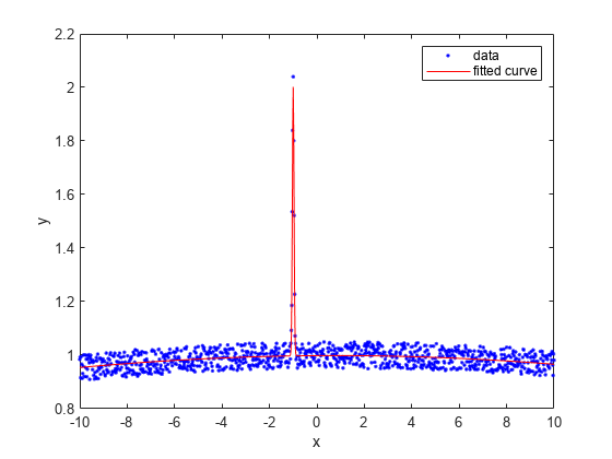
此拟合效果更佳。您可以通过为拟合选项对象中的其他属性指定合理值来进一步改善拟合。

复制并合并拟合选项

打开实时脚本

创建拟合选项并设置下界。

options = fitoptions('gauss2', 'Lower', [0 -Inf 0 0 -Inf 0])

options = 
  nlsqoptions with properties:

          StartPoint: []
           Algorithm: 'Trust-Region'
       DiffMinChange: 1.0000e-08
       DiffMaxChange: 0.1000
             Display: 'Notify'
         MaxFunEvals: 600
             MaxIter: 400
              TolFun: 1.0000e-06
                TolX: 1.0000e-06
               Lower: [0 -Inf 0 0 -Inf 0]
               Upper: []
    ConstraintPoints: []
              TolCon: 1.0000e-06
              Robust: 'Off'
           Normalize: 'off'
             Exclude: []
             Weights: []
              Method: 'NonlinearLeastSquares'

创建拟合选项的新副本，并修改稳健参数。

newoptions = fitoptions(options, 'Robust','Bisquare')

newoptions = 
  nlsqoptions with properties:

          StartPoint: []
           Algorithm: 'Trust-Region'
       DiffMinChange: 1.0000e-08
       DiffMaxChange: 0.1000
             Display: 'Notify'
         MaxFunEvals: 600
             MaxIter: 400
              TolFun: 1.0000e-06
                TolX: 1.0000e-06
               Lower: [0 -Inf 0 0 -Inf 0]
               Upper: []
    ConstraintPoints: []
              TolCon: 1.0000e-06
              Robust: 'Bisquare'
           Normalize: 'off'
             Exclude: []
             Weights: []
              Method: 'NonlinearLeastSquares'

合并拟合选项。

options2 = fitoptions(options, newoptions)

options2 = 
  nlsqoptions with properties:

          StartPoint: []
           Algorithm: 'Trust-Region'
       DiffMinChange: 1.0000e-08
       DiffMaxChange: 0.1000
             Display: 'Notify'
         MaxFunEvals: 600
             MaxIter: 400
              TolFun: 1.0000e-06
                TolX: 1.0000e-06
               Lower: [0 -Inf 0 0 -Inf 0]
               Upper: []
    ConstraintPoints: []
              TolCon: 1.0000e-06
              Robust: 'Bisquare'
           Normalize: 'off'
             Exclude: []
             Weights: []
              Method: 'NonlinearLeastSquares'

更改自定义模型拟合选项

打开实时脚本

创建一个线性模型拟合类型。

lft = fittype({'x','sin(x)','1'})

lft = 
     Linear model:
     lft(a,b,c,x) = a*x + b*sin(x) + c

获取拟合类型 lft 的拟合选项。

fo = fitoptions(lft)

fo = 
  llsqoptions with properties:

               Lower: []
               Upper: []
    ConstraintPoints: []
              TolCon: 1.0000e-06
              Robust: 'Off'
           Normalize: 'off'
             Exclude: []
             Weights: []
              Method: 'LinearLeastSquares'

设置归一化拟合选项。

fo.Normalize = 'on'

fo = 
  llsqoptions with properties:

               Lower: []
               Upper: []
    ConstraintPoints: []
              TolCon: 1.0000e-06
              Robust: 'Off'
           Normalize: 'on'
             Exclude: []
             Weights: []
              Method: 'LinearLeastSquares'

输入参数

全部折叠

`libraryModelName` — 要拟合的库模型
字符向量 | 字符串标量

要拟合的库模型，指定为字符向量或字符串标量。下表列出了一些常见示例。

库模型名称	描述
`'poly1'`	线性多项式曲线
`'poly11'`	线性多项式曲面
`'poly2'`	二次多项式曲线
`'linearinterp'`	分段线性插值
`'cubicinterp'`	分段三次插值
`'smoothingspline'`	平滑样条（曲线）
`'lowess'`	局部线性回归（曲面）
`'log10'`	以 10 为底的对数曲线
`'logistic4'`	四参数逻辑曲线

有关库模型名称的列表，请参阅模型名称和方程。

示例: 'poly2'

数据类型: char | string

`fitType` — 要拟合的模型类型
`fittype`

要拟合的模型类型，指定为用 fittype 函数构造的 fittype。可将此项与拟合选项结合用于自定义模型。

`fitOptions` — 算法选项
`fitoptions`

算法选项，指定为使用 fitoptions 函数创建的 fitoptions 对象。

`options1` — 要合并的算法选项
`fitoptions`

要合并的算法选项，使用 fitoptions 函数构造。

`options2` — 要合并的算法选项
`fitoptions`

要合并的算法选项，使用 fitoptions 函数构造。

名称-值参数

全部展开

将可选参量对组指定为 Name1=Value1,...,NameN=ValueN，其中 Name 是参量名称，Value 是对应的值。名称-值参量必须出现在其他参量之后，但对各个参量对组的顺序没有要求。

在 R2021a 之前，使用逗号分隔每个名称和值，并用引号将 Name 引起来。

示例: 'Method','NonlinearLeastSquares','Lower',[0,0],'Upper',[Inf,max(x)],'Startpoint',[1 1] 指定拟合方法、边界和起点。

所有拟合方法的选项

全部展开

`Normalize` — 中心化和缩放数据的选项
`'off'` (默认) | `'on'`

用于中心化和缩放数据的选项，指定为由 'Normalize' 和 'on' 或 'off' 组成的以逗号分隔的对组。

数据类型: char

`Exclude` — 要从拟合中排除的点
表达式 | 索引向量 | 逻辑向量 | 空

要从拟合中排除的点，指定为由 'Exclude' 和以下项之一组成的以逗号分隔的对组：

描述逻辑向量的表达式，例如 x > 10。
对要排除的点进行索引的整数组成的向量，例如 [1 10 25]。
所有数据点的逻辑向量，其中 true 表示离群值，由 excludedata 创建。

有关示例，请参阅 fit。

`Weights` — 拟合的权重
[ ] (默认) | 向量

拟合的权重，指定为以逗号分隔的对组，其中包括 'Weights' 和与数据点数大小相同的向量。

数据类型: double

`Method` — 拟合方法
`'None'` (默认) | `'NearestInterpolant` | `'LinearInterpolant'` | `'PchipInterpolant'` | `CubicSplineInterpolant'` | ...

拟合方法，指定为以逗号分隔的对组，其中包含 'Method' 和下表中的拟合方法之一。

拟合方法	描述
`'NearestInterpolant'`	最近邻点插值
`'LinearInterpolant'`	线性插值
`'PchipInterpolant'`	分段三次埃尔米特插值（仅限曲线）
`'CubicSplineInterpolant'`	三次样条插值
`'BiharmonicInterpolant'`	双调和曲面插值
`'SmoothingSpline'`	平滑样条
`'LowessFit'`	Lowess 平滑（仅限曲面）
`'LinearLeastSquares'`	线性最小二乘
`'NonlinearLeastSquares'`	非线性最小二乘

数据类型: char | string

插值选项

全部展开

`ExtrapolationMethod` — 外插方法
`"auto"` (默认) | `"none"` | `"linear"` | `"nearest"` | `"thinplate"` | `"biharmonic"` | `"pchip"` | `"cubic"`

插值拟合的外插方法，指定为以下值之一：

值	描述	支持的拟合
`"auto"`	所有插值拟合类型的默认值。将 `ExtrapolationMethod` 设置为 `"auto"`，以便在使用 `fit` 函数时自动指定外插方法。	所有插值拟合类型和 `cubicspline` 曲线拟合
`"none"`	无外插。当您将 `fitOptions` 与 `fit` 函数结合使用来计算凸包之外的查询点时，`fit` 将返回 `NaN`。	曲线拟合 - `cubicspline` 和 `pchipinterp` 曲面拟合 - `naturalinterp` 曲线拟合和曲面拟合 - `cubicinterp`、`linearinterp` 和 `nearestinterp`
`"linear"`	基于边界梯度的线性外插	曲面拟合 - `cubicinterp`、`nearestinterp` 和 `naturalinterp` 曲线拟合和曲面拟合 - `linearinterp`
`"nearest"`	最近邻点外插。这种方法的计算结果为拟合数据凸包边界上最近点的值。	曲线拟合 - `cubicspline` 和 `pchipinterp` 曲面拟合 - `naturalinterp` 曲线拟合和曲面拟合 - `cubicinterp`、`linearinterp` 和 `nearestinterp`
`"thinplate"`	薄板样条外插。这种方法可将薄板内插样条扩展到拟合数据的凸包之外。有关详细信息，请参阅 `tpaps`。	曲面拟合 - `thinplateinterp`
`"biharmonic"`	双调和样条外插。这种方法可将双调和内插样条扩展到拟合数据的凸包之外。	曲面拟合 - `biharmonicinterp`
`"pchip"`	分段三次埃尔米特插值多项式 (PCHIP) 外插。这种方法可将保形 PCHIP 扩展到拟合数据的凸包之外。有关详细信息，请参阅 `pchip`。	曲线拟合 - `pchipinterp`
`"cubic"`	三次样条外插。这种方法可将三次插值样条扩展到拟合数据的凸包之外。	曲线拟合 - `cubicinterp` 和 `cubicspline`

数据类型: char | string

平滑选项

全部展开

`SmoothingParam` — 平滑参数
范围 (0,1) 中的标量值

平滑参数，指定为以逗号分隔的对组，其中包含 'SmoothingParam' 和介于 0 和 1 之间的标量值。默认值取决于数据集。仅当 Method 为 SmoothingSpline 时可用。有关详细信息，请参阅About Smoothing Splines。

数据类型: double

`Span` — 用于局部回归的数据点的比例
0.25 (默认) | 范围 (0,1) 中的标量值

用于局部回归的数据点的比例，指定为以逗号分隔的对组，其中包含 'Span' 和介于 0 和 1 之间的标量值。仅当 Method 为 LowessFit 时可用。

数据类型: double

线性和非线性最小二乘选项

全部展开

`Robust` — 稳健线性最小二乘拟合方法
`'off'` (默认) | `'LAR'` | `'Bisquare'`

稳健线性最小二乘拟合方法，指定为以逗号分隔的对组，其中包含 'Robust' 和以下值之一：

'LAR' 指定最小绝对残差方法。
'Bisquare' 指定 bisquare 权重方法。

当 Method 为 LinearLeastSquares 或 NonlinearLeastSquares 时可用。

数据类型: char

`Lower` — 要拟合的系数的下界
[ ] (默认) | 向量

要拟合的系数的下界，指定为以逗号分隔的对组，其中包含 'Lower' 和向量。默认值为一个空向量，表示拟合不受下界的约束。如果指定边界，则向量长度必须等于系数数目。使用 coeffnames 函数找出向量值中系数项的顺序。有关示例，请参阅 fit。各个无约束下界可以由 -Inf 指定。

当 Method 为 LinearLeastSquares 或 NonlinearLeastSquares 时可用。

数据类型: double

`Upper` — 要拟合的系数的上界
[ ] (默认) | 向量

要拟合的系数的上界，指定为以逗号分隔的对组，其中包含 'Upper' 和向量。默认值为一个空向量，表示拟合不受上界的约束。如果指定边界，则向量长度必须等于系数数目。使用 coeffnames 函数找出向量值中系数项的顺序。有关示例，请参阅 fit。各个无约束上界可以由 +Inf 指定。

当 Method 为 LinearLeastSquares 或 NonlinearLeastSquares 时可用。

数据类型: logical

`ConstraintPoints` — 拟合要经过的点
`[]` (默认) | 数值矩阵

自 R2025a 起

拟合要经过的点，指定为 nx2 数值矩阵（对于曲线），或 nx3 数值矩阵（对于曲面）。每行表示一个约束点，而每列表示该点的 x、y 或 z 坐标。约束点的数目不能大于指定 fitType 中系数的数目。您可以使用 numcoeffs 查找拟合类型中系数的数目。如果指定最大约束点数，则只能得到一个解，且该解与输入数据无关。

注意

您必须安装有 Optimization Toolbox™，才能使用约束点来拟合模型。

当 Method 为 LinearLeastSquares 或 NonlinearLeastSquares 时可用。

示例: [0 0; 1 5]

数据类型: double

`TolCon` — 约束点的容差
10^–6 (默认) | 非负数值标量

自 R2025a 起

约束点的容差，指定为非负数值标量。这是在发生违反约束之前，所提供约束点与拟合实际经过的点之间的绝对数值差异的上界。

如果 ConstraintPoints 名称-值参量未指定，则 TolCon 无效。

注意

TolCon 的运算原理不同于其他容差。即使满足 TolCon 条件，求解器仍继续运行，除非由于其他原因停止运行。求解器不会仅仅因为满足 TolCon 就停止。

当 Method 为 LinearLeastSquares 或 NonlinearLeastSquares 时可用。

数据类型: double

非线性最小二乘选项

全部展开

`StartPoint` — 系数的初始值
[ ] (默认) | 向量

系数的初始值，指定为以逗号分隔的对组，其中包含 'StartPoint' 和向量。使用 coeffnames 函数找出向量值中系数项的顺序。有关示例，请参阅 fit。

如果起点（空向量的默认值）未传递给 fit 函数，则某些库模型的起点是通过启发式方法确定的。对于有理和威布尔模型，以及所有自定义的非线性模型，工具箱从区间 (0,1) 中均匀随机地选择系数的默认初始值。因此，使用相同数据和模型的多个拟合可能导致不同的拟合系数。要避免这种情况，请为 StartPoint 属性指定一个向量值作为系数初始值。