Smoothing Splines

About Smoothing Splines

If your data is noisy, you might want to fit it using a smoothing spline. Alternatively, you can use one of the smoothing methods described in Filtering and Smoothing Data.

The smoothing spline s is constructed for the specified smoothing parameter p and the specified weights w_i. The smoothing spline minimizes

$p {\sum_{i} w_{i} {(y_{i} - s (x_{i}))}^{2} + (1 - p) \int (\frac{d^{2} s}{d x^{2}})}^{2} d x$

If the weights are not specified, they are assumed to be 1 for all data points.

p is defined between 0 and 1. p = 0 produces a least-squares straight-line fit to the data, while p = 1 produces a cubic spline interpolant. If you do not specify the smoothing parameter, it is automatically selected in the “interesting range.” The interesting range of p is often near 1/(1+h³/6) where h is the average spacing of the data points, and the interesting range is typically much smaller than the allowed range [0,1] of the parameter p. Because smoothing splines have an associated smoothing parameter, you might consider these fits to be parametric in that sense. However, smoothing splines are also piecewise polynomials like cubic spline or shape-preserving interpolants and are considered a nonparametric fit type in this guide.

Note

The smoothing spline algorithm is based on the csaps function.

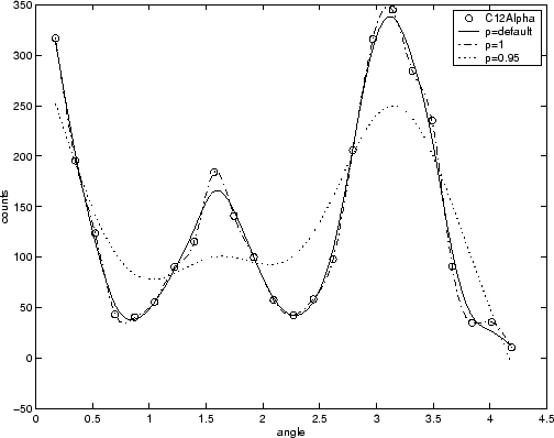
The nuclear reaction data from the file carbon12alpha.mat is shown here with three smoothing spline fits. The default smoothing parameter (p = 0.99) produces the smoothest curve. The cubic spline curve (p = 1) goes through all the data points, but is not quite as smooth. The third curve (p = 0.95) misses the data by a wide margin and illustrates how small the “interesting range” of p can be.

Axes with three curves and a legend. The horizontal axis is labeled angle and the vertical axis is labeled counts.

Select Smoothing Spline Fit Interactively

Load the data at the MATLAB^® command line.
```
load carbon12alpha
```
Open the Curve Fitter app.
```
curveFitter
```
Alternatively, on the Apps tab, in the Math, Statistics and Optimization group, click Curve Fitter.
On the Curve Fitter tab, in the Data section, click Select Data. In the Select Fitting Data dialog box, select angle as the X data value and counts as the Y data value. For details, see Select Data to Fit in Curve Fitter App.
On the Curve Fitter tab, in the Fit Type section, click the arrow to open the gallery, and click Smoothing Spline in the Smoothing group.
In the Fit Options pane, you can specify the Smoothing Parameter value.
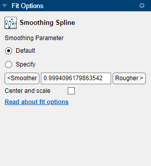
The default Smoothing Parameter value is close to 1. The app tries to select a default value appropriate for your data. You can change the Smoothing Parameter value by doing one of the following:
- To create a smoother fit further from the data, click the < Smoother button repeatedly until the plot shows the smoothness you want.
- To create a rougher fit closer to the data, click the Rougher > button until you are satisfied with the plot.
- Alternatively, specify any value from 0 to 1 for the smoothing parameter. A value of 0 produces a linear polynomial fit (a least-squares straight-line fit to the data), while 1 produces a piecewise cubic polynomial fit that passes through all the data points (a cubic spline interpolant). For the carbon12alpha data set, try Smoothing Parameter values 1 and 0.95.
- Click Default to return to the initial value.

Fit Smoothing Spline Models Using the `fit` Function

Open Live Script

This example shows how to use the fit function to fit a smoothing spline model to data.

Fit a Smoothing Spline Model

Load data and fit a smoothing spline model by specifying 'smoothingspline' when calling the fit function.

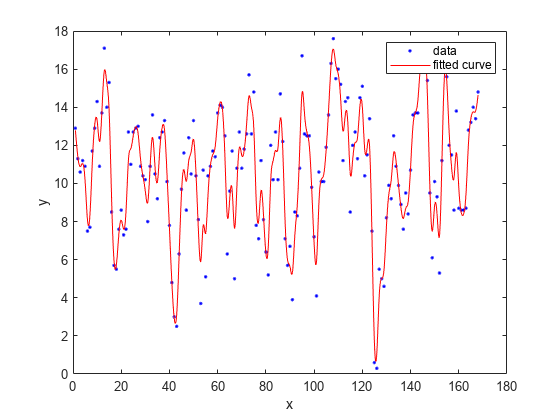
load enso
f = fit(month,pressure,'smoothingspline');
plot(f,month,pressure)

Figure contains an axes object. The axes object with xlabel x, ylabel y contains 2 objects of type line. One or more of the lines displays its values using only markers These objects represent Data, Fitted curve.

View Calculated Smoothing Parameter

Create the model again and use the third output argument to view the calculated smoothing parameter. The smoothing parameter is the p value in the out structure. The default value depends on the data set.

[f,gof,out] = fit(month,pressure,'smoothingspline');

out.p

ans = 
0.9000

Specify Smoothing Parameter using 'SmoothingParam'

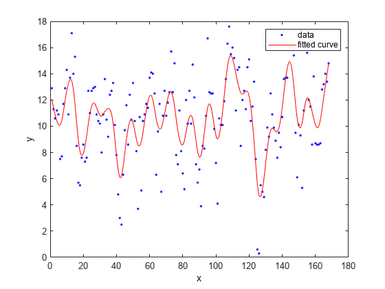
Specify the smoothing parameter for a new fit with the 'SmoothingParam' option. Its value must be between 0 and 1.

f = fit(month,pressure,'smoothingspline','SmoothingParam',0.07);
plot(f,month,pressure)

Specify Smoothing Parameter using fitoptions

Alternatively, use fitoptions to specify a smoothing parameter before fitting.

options = fitoptions('Method','Smooth','SmoothingParam',0.07);
[f,gof,out] = fit(month,pressure,'smooth',options);
out.p

ans = 
0.0700

For an alternative to 'smoothingspline', you can use the csaps cubic smoothing spline function or other spline functions that allow greater control over what you can create. See Introducing Spline Fitting.

Compare Cubic and Smoothing Spline Fit Using Curve Fitter

This example compares a cubic spline interpolant fit and a smoothing spline fit using the Curve Fitter app.

Create the data x and y.

x = (4*pi)*[0 1 rand(1,25)]; 
y = sin(x) + .2*(rand(size(x))-.5);

Open the Curve Fitter app.
```
curveFitter
```
Alternatively, on the Apps tab, in the Math, Statistics and Optimization group, click Curve Fitter.
On the Curve Fitter tab, in the Data section, click Select Data. In the Select Fitting Data dialog box, select x as the X data value and y as the Y data value.
On the Curve Fitter tab, in the Fit Type section, click the arrow to open the gallery, and click Interpolant in the Interpolation group.
In the Fit Options pane, specify the Interpolation Method as Cubic spline. The Curve Fitter app fits and plots the cubic spline interpolant.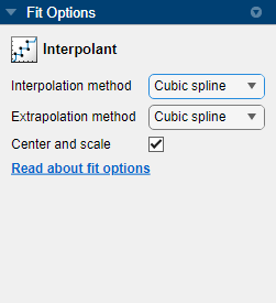
Rename the fit. In the Table Of Fits pane, double-click the Fit Name value and enter CubicSplineFit.
View the Results pane. Some goodness-of-fit statistics, such as RMSE, are not defined for Interpolant fits and their value is NaN.
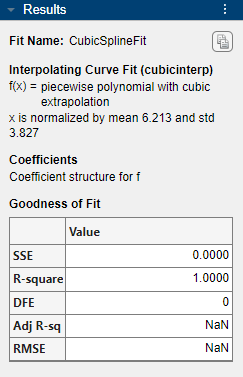
A cubic spline interpolation is defined as a piecewise polynomial that results in a structure of coefficients (p). The number of “pieces” in the structure is one less than the number of fitted data points, and the number of coefficients for each piece is four because the polynomial degree is three. You can examine the coefficient structure p if you export your fit to the workspace by entering CubicSplineFit.p. For more information on the coefficient structure, see Constructing and Working with ppform Splines.
Create another fit to compare. Right-click the existing fit CubicSplineFit on the Table Of Fits tab and select Duplicate "CubicSplineFit". Rename the new fit to SmoothingSplineFit.
On the Curve Fitter tab, in the Fit Type section, select a Smoothing Spline fit.
In the Fit Options pane, the Smoothing Parameter defines the level of smoothness. The app calculates the Smoothing Parameter depending on the data set. For this data set, the default Smoothing Parameter is close to 1, indicating that the smoothing spline is nearly cubic and comes very close to passing through each data point.
You can change the level of smoothing by specifying Smoothing Parameter as a nonnegative scalar in the range [0 1]. Specify Smoothing Parameter as 0 to create a linear polynomial fit. Specify Smoothing Parameter as 1 to create a piecewise cubic polynomial fit that passes through all the data points.
See the Results pane for numerical results of the smoothing spline fit.
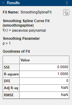
Compare the plots for the two fits (cubic spline interpolant fit and smoothing spline fit), which you created. The two fits are similar for interior points, but diverge at the end points.