Filtering and Smoothing Data

About Data Filtering and Smoothing

This topic explains how to smooth response data using this function. With the smooth function, you can use optional methods for moving average, Savitzky-Golay filters, and local regression with and without weights and robustness (lowess, loess, rlowess and rloess). See smoothdata for more functionality, including support for matrices, tables, and timetables, as well as moving median and Gaussian methods.

Moving Average Filtering

A moving average filter smooths data by replacing each data point with the average of the neighboring data points defined within the span. This process is equivalent to lowpass filtering with the response of the smoothing given by the difference equation

$y_{s} (i) = \frac{1}{2 N + 1} (y (i + N) + y (i + N - 1) + ... + y (i - N))$

where y_s(i) is the smoothed value for the ith data point, N is the number of neighboring data points on either side of y_s(i), and 2N+1 is the span.

The moving average smoothing method used by Curve Fitting Toolbox™ follows these rules:

The span must be odd.
The data point to be smoothed must be at the center of the span.
The span is adjusted for data points that cannot accommodate the specified number of neighbors on either side.
The end points are not smoothed because a span cannot be defined.

Note that you can use filter function to implement difference equations such as the one shown above. However, because of the way that the end points are treated, the toolbox moving average result will differ from the result returned by filter. Refer to Difference Equations and Filtering for more information.

For example, suppose you smooth data using a moving average filter with a span of 5. Using the rules described above, the first four elements of y_s are given by

y_s(1) = y(1)
y_s(2) = (y(1)+y(2)+y(3))/3
y_s(3) = (y(1)+y(2)+y(3)+y(4)+y(5))/5
y_s(4) = (y(2)+y(3)+y(4)+y(5)+y(6))/5

Note that y_s(1), y_s(2), ... ,y_s(end) refer to the order of the data after sorting, and not necessarily the original order.

The smoothed values and spans for the first four data points of a generated data set are shown below.

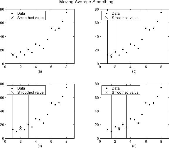
Plot (a) indicates that the first data point is not smoothed because a span cannot be constructed. Plot (b) indicates that the second data point is smoothed using a span of three. Plots (c) and (d) indicate that a span of five is used to calculate the smoothed value.

Savitzky-Golay Filtering

Savitzky-Golay filtering can be thought of as a generalized moving average. You derive the filter coefficients by performing an unweighted linear least-squares fit using a polynomial of a given degree. For this reason, a Savitzky-Golay filter is also called a digital smoothing polynomial filter or a least-squares smoothing filter. Note that a higher degree polynomial makes it possible to achieve a high level of smoothing without attenuation of data features.

The Savitzky-Golay filtering method is often used with frequency data or with spectroscopic (peak) data. For frequency data, the method is effective at preserving the high-frequency components of the signal. For spectroscopic data, the method is effective at preserving higher moments of the peak such as the line width. By comparison, the moving average filter tends to filter out a significant portion of the signal's high-frequency content, and it can only preserve the lower moments of a peak such as the centroid. However, Savitzky-Golay filtering can be less successful than a moving average filter at rejecting noise.

The Savitzky-Golay smoothing method used by Curve Fitting Toolbox software follows these rules:

The span must be odd.
The polynomial degree must be less than the span.
The data points are not required to have uniform spacing.
Normally, Savitzky-Golay filtering requires uniform spacing of the predictor data. However, the Curve Fitting Toolbox algorithm supports nonuniform spacing. Therefore, you are not required to perform an additional filtering step to create data with uniform spacing.

The plot shown below displays generated Gaussian data and several attempts at smoothing using the Savitzky-Golay method. The data is very noisy and the peak widths vary from broad to narrow. The span is equal to 5% of the number of data points.

The figure shows three plots with labeled a, b, and c. Plot a shows a curve with many peaks and troughs. Plot b shows a curve that is much smoother than the curve in axes a. Plot c shows a curve that is less smooth than the curve in plot b.

Plot (a) shows the noisy data. To more easily compare the smoothed results, plots (b) and (c) show the data without the added noise.

Plot (b) shows the result of smoothing with a quadratic polynomial. Notice that the method performs poorly for the narrow peaks. Plot (c) shows the result of smoothing with a quartic polynomial. In general, higher degree polynomials can more accurately capture the heights and widths of narrow peaks, but can do poorly at smoothing wider peaks.

Lowess and Loess

The names “lowess” and “loess” are derived from the term “locally weighted scatter plot smooth,” as both methods use locally weighted linear regression to smooth data.

The smoothing process is considered local because, like the moving average method, each smoothed value is determined by neighboring data points defined within the span. The process is weighted because a regression weight function is defined for the data points contained within the span. In addition to the regression weight function, you can use a robust weight function, which makes the process resistant to outliers. Finally, the methods are differentiated by the model used in the regression: lowess uses a linear polynomial, while loess uses a quadratic polynomial.

The local regression smoothing methods used by Curve Fitting Toolbox software follow these rules:

The span can be even or odd.
You can specify the span as a percentage of the total number of data points in the data set. For example, a span of 0.1 uses 10% of the data points.

The Local Regression Method

The local regression smoothing process follows these steps for each data point:

Compute the regression weights for each data point in the span. The weights are given by the tricube function shown below.
$w_{i} = {(1 - {| \frac{x - x_{i}}{d (x)} |}^{3})}^{3}$
x is the predictor value associated with the response value to be smoothed, x_i are the nearest neighbors of x as defined by the span, and d(x) is the distance along the abscissa from x to the most distant predictor value within the span. The weights have these characteristics:
- The data point to be smoothed has the largest weight and the most influence on the fit.
- Data points outside the span have zero weight and no influence on the fit.
A weighted linear least-squares regression is performed. For lowess, the regression uses a first degree polynomial. For loess, the regression uses a second degree polynomial.
The smoothed value is given by the weighted regression at the predictor value of interest.

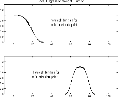
If the smooth calculation involves the same number of neighboring data points on either side of the smoothed data point, the weight function is symmetric. However, if the number of neighboring points is not symmetric about the smoothed data point, then the weight function is not symmetric. Note that unlike the moving average smoothing process, the span never changes. For example, when you smooth the data point with the smallest predictor value, the shape of the weight function is truncated by one half, the leftmost data point in the span has the largest weight, and all the neighboring points are to the right of the smoothed value.

The weight function for an end point and for an interior point is shown below for a span of 31 data points.

The figure shows two plots. On the left side of the top plot, a downward sloping curve is located between two vertical lines. The top plot includes the text "The weight function for the leftmost data point". On the center-right of the bottom plot, a bell-shaped curve is located between two vertical lines. The bottom plot includes the text "The weight function for an interior data point".

Using the lowess method with a span of five, the smoothed values and associated regressions for the first four data points of a generated data set are shown below.

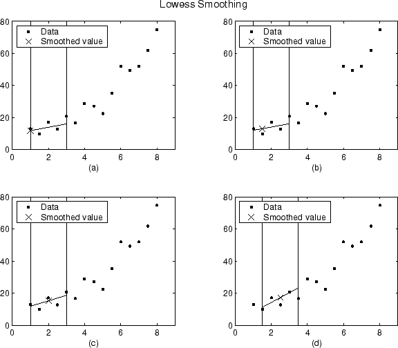
Notice that the span does not change as the smoothing process progresses from data point to data point. However, depending on the number of nearest neighbors, the regression weight function might not be symmetric about the data point to be smoothed. In particular, plots (a) and (b) use an asymmetric weight function, while plots (c) and (d) use a symmetric weight function.

For the loess method, the graphs would look the same except the smoothed value would be generated by a second-degree polynomial.

Robust Local Regression

If your data contains outliers, the smoothed values can become distorted, and not reflect the behavior of the bulk of the neighboring data points. To overcome this problem, you can smooth the data using a robust procedure that is not influenced by a small fraction of outliers. For a description of outliers, refer to Residual Analysis.

Curve Fitting Toolbox software provides a robust version for both the lowess and loess smoothing methods. These robust methods include an additional calculation of robust weights, which is resistant to outliers. The robust smoothing procedure follows these steps:

Calculate the residuals from the smoothing procedure described in the previous section.
Compute the robust weights for each data point in the span. The weights are given by the bisquare function,
$w_{i} = {\begin{matrix} {(1 - {(r_{i} / 6 M A D)}^{2})}^{2}, & | r i | < 6 M A D, \\ 0, & | r i | \geq 6 M A D, \end{matrix}$
where r_i is the residual of the ith data point produced by the regression smoothing procedure, and MAD is the median absolute deviation of the residuals,
$M A D = median (| r |) .$
The median absolute deviation is a measure of how spread out the residuals are. If r_i is small compared to 6MAD, then the robust weight is close to 1. If r_i is greater than 6MAD, the robust weight is 0 and the associated data point is excluded from the smooth calculation.
Smooth the data again using the robust weights. The final smoothed value is calculated using both the local regression weight and the robust weight.
Repeat the previous two steps for a total of five iterations.

The smoothing results of the lowess procedure are compared below to the results of the robust lowess procedure for a generated data set that contains a single outlier. The span for both procedures is 11 data points.

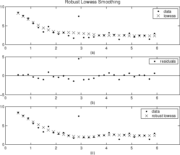
The figure shows three plots labeled a, b, and c. Plots a and c have legends in which dots represent the data and x's represent the smoothed values. Plot a shows dots with nearby x's. The x's follow the dots less closely in a region where a single dot is much higher than the others. Plot b shows a residuals plot. Plot c shows the x's following the dots more closely relative to axis a.

Plot (a) shows that the outlier influences the smoothed value for several nearest neighbors. Plot (b) suggests that the residual of the outlier is greater than six median absolute deviations. Therefore, the robust weight is zero for this data point. Plot (c) shows that the smoothed values neighboring the outlier reflect the bulk of the data.

Example: Smoothing Data

Load the data in count.dat:

load count.dat

The 24-by-3 array count contains traffic counts at three intersections for each hour of the day.

First, use a moving average filter with a 5-hour span to smooth all of the data at once (by linear index) :

c = smooth(count(:));
C1 = reshape(c,24,3);

Plot the original data and the smoothed data:

subplot(3,1,1)
plot(count,':');
hold on
plot(C1,'-');
title('Smooth C1 (All Data)')

Second, use the same filter to smooth each column of the data separately:

C2 = zeros(24,3);
for I = 1:3,
    C2(:,I) = smooth(count(:,I));
end

Again, plot the original data and the smoothed data:

subplot(3,1,2)
plot(count,':');
hold on
plot(C2,'-');
title('Smooth C2 (Each Column)')

Plot the difference between the two smoothed data sets:

subplot(3,1,3)
plot(C2 - C1,'o-')
title('Difference C2 - C1')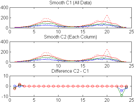

Note the additional end effects from the 3-column smooth.

Example: Smoothing Data Using Loess and Robust Loess

Create noisy data with outliers:

x = 15*rand(150,1); 
y = sin(x) + 0.5*(rand(size(x))-0.5);
y(ceil(length(x)*rand(2,1))) = 3;

Smooth the data using the loess and rloess methods with a span of 10%:

yy1 = smooth(x,y,0.1,'loess');
yy2 = smooth(x,y,0.1,'rloess');

Plot original data and the smoothed data.

[xx,ind] = sort(x);
subplot(2,1,1)
plot(xx,y(ind),'b.',xx,yy1(ind),'r-')
set(gca,'YLim',[-1.5 3.5])
legend('Original Data','Smoothed Data Using ''loess''',...
       'Location','NW')
subplot(2,1,2)
plot(xx,y(ind),'b.',xx,yy2(ind),'r-')
set(gca,'YLim',[-1.5 3.5])
legend('Original Data','Smoothed Data Using ''rloess''',...
       'Location','NW')

The figure shows two plots. Both plots contain legends indicating that the data is represented by points and smoothed data is represented by curves. The curve in the top plot was calculated using the loess method. The curve in the bottom plot was smoothed using rloess. The curve in the bottom plot is smoother than the curve it the top plot.

Note that the outliers have less influence on the robust method.