Design NARMA-L2 Neural Controller in Simulink

The neurocontroller described in this section is referred to by two different names: feedback linearization control and NARMA-L2 control. It is referred to as feedback linearization when the plant model has a particular form (companion form). It is referred to as NARMA-L2 control when the plant model can be approximated by the same form. The central idea of this type of control is to transform nonlinear system dynamics into linear dynamics by canceling the nonlinearities. This section begins by presenting the companion form system model and showing how you can use a neural network to identify this model. Then it describes how the identified neural network model can be used to develop a controller. This is followed by an example of how to use the NARMA-L2 Control block, which is contained in the Deep Learning Toolbox™ blockset.

Identification of the NARMA-L2 Model

As with model predictive control, the first step in using feedback linearization (or NARMA-L2) control is to identify the system to be controlled. You train a neural network to represent the forward dynamics of the system. The first step is to choose a model structure to use. One standard model that is used to represent general discrete-time nonlinear systems is the nonlinear autoregressive-moving average (NARMA) model:

$y (k + d) = N [y (k), y (k - 1), \dots, y (k - n + 1), u (k), u (k - 1), \dots, u (k - n + 1)]$

where u(k) is the system input, and y(k) is the system output. For the identification phase, you could train a neural network to approximate the nonlinear function N. This is the identification procedure used for the NN Predictive Controller.

If you want the system output to follow some reference trajectory
y(k + d) = y_r(k + d), the next step is to develop a nonlinear controller of the form:

$u (k) = G [y (k), y (k - 1), \dots, y (k - n + 1), y_{r} (k + d), u (k - 1), \dots, u (k - m + 1)]$

The problem with using this controller is that if you want to train a neural network to create the function G to minimize mean square error, you need to use dynamic backpropagation ([NaPa91] or [HaJe99]). This can be quite slow. One solution, proposed by Narendra and Mukhopadhyay [NaMu97], is to use approximate models to represent the system. The controller used in this section is based on the NARMA-L2 approximate model:

$\begin{matrix} \hat{y} (k + d) = f [y (k), y (k - 1), \dots, y (k - n + 1), u (k - 1), \dots, u (k - m + 1)] \\ + g [y (k), y (k - 1), \dots, y (k - n + 1), u (k - 1), \dots, u (k - m + 1)] \cdot u (k) \end{matrix}$

This model is in companion form, where the next controller input u(k) is not contained inside the nonlinearity. The advantage of this form is that you can solve for the control input that causes the system output to follow the reference y(k + d) = y_r(k + d). The resulting controller would have the form

$u (k) = \frac{y_{r} (k + d) - f [y (k), y (k - 1), \dots, y (k - n + 1), u (k - 1), \dots, u (k - n + 1)]}{g [y (k), y (k - 1), \dots, y (k - n + 1), u (k - 1), \dots, u (k - n + 1)]}$

Using this equation directly can cause realization problems, because you must determine the control input u(k) based on the output at the same time, y(k). So, instead, use the model

$\begin{matrix} y (k + d) = f [y (k), y (k - 1), \dots, y (k - n + 1), u (k), u (k - 1), \dots, u (k - n + 1)] \\ + g [y (k), \dots, y (k - n + 1), u (k), \dots, u (k - n + 1)] \cdot u (k + 1) \end{matrix}$

where d ≥ 2. The following figure shows the structure of a neural network representation.

NARMA-L2 Controller

Using the NARMA-L2 model, you can obtain the controller

$u (k + 1) = \frac{y_{r} (k + d) - f [y (k), \dots, y (k - n + 1), u (k), \dots, u (k - n + 1)]}{g [y (k), \dots, y (k - n + 1), u (k), \dots, u (k - n + 1)]}$

which is realizable for d ≥ 2. The following figure is a block diagram of the NARMA-L2 controller.

This controller can be implemented with the previously identified NARMA-L2 plant model, as shown in the following figure.

Use the NARMA-L2 Controller Block

This section shows how the NARMA-L2 controller is trained. The first step is to copy the NARMA-L2 Controller block from the Deep Learning Toolbox block library to the Simulink^® Editor. See the Simulink documentation if you are not sure how to do this. This step is skipped in the following example.

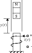
An example model is provided with the Deep Learning Toolbox software to show the use of the NARMA-L2 controller. In this example, the objective is to control the position of a magnet suspended above an electromagnet, where the magnet is constrained so that it can only move in the vertical direction, as in the following figure.

The equation of motion for this system is

$\frac{d^{2} y (t)}{d t^{2}} = - g + \frac{α}{M} \frac{i^{2} (t)}{y (t)} - \frac{β}{M} \frac{d y (t)}{d t}$

where y(t) is the distance of the magnet above the electromagnet, i(t) is the current flowing in the electromagnet, M is the mass of the magnet, and g is the gravitational constant. The parameter β is a viscous friction coefficient that is determined by the material in which the magnet moves, and α is a field strength constant that is determined by the number of turns of wire on the electromagnet and the strength of the magnet.

To run this example:

Start MATLAB^®.
Type narmamaglev in the MATLAB Command Window. This command opens the Simulink Editor with the following model. The NARMA-L2 Control block is already in the model.
Double-click the NARMA-L2 Controller block. This opens the following window. This window enables you to train the NARMA-L2 model. There is no separate window for the controller, because the controller is determined directly from the model, unlike the model predictive controller.
This window works the same as the other Plant Identification windows, so the training process is not repeated. Instead, simulate the NARMA-L2 controller.
Return to the Simulink Editor and start the simulation by choosing the menu option Simulation > Run. As the simulation runs, the plant output and the reference signal are displayed, as in the following figure.