Use Experiment Manager in the Cloud with MATLAB Deep Learning Container

Classification of CIFAR-10 Image Data with Experiment Manager in the Cloud

To get started with Experiment Manager for a classification network example, first download the CIFAR-10 training data to the MATLAB® Deep Learning Container. A simple way to do so is to use the downloadCIFARToFolders function, attached to this example as a supporting file. To access this file, open the example as a live script. The following code downloads the data set to your current directory.

directory = pwd;
[locationCifar10Train,locationCifar10Test] = downloadCIFARToFolders(directory);

Downloading CIFAR-10 data set...done.
Copying CIFAR-10 to folders...done.

Next, open Experiment Manager by running experimentManager in the MATLAB command window or by opening the Experiment Manager App from the Apps tab.

experimentManager

In Experiment Manager, select New and then Project. After a new window opens, select Blank Project and then Built-In Training (trainnet).

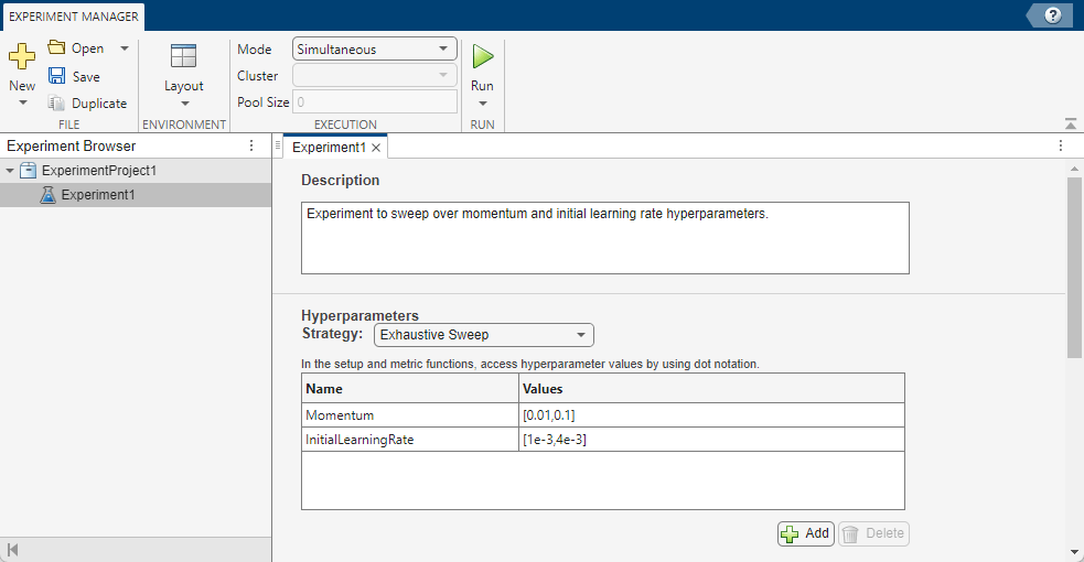
Hyperparameters

In the hyperparameters section, add two new parameters. Name the first Momentum with values [0.01,0.1] and the second InitialLearningRate with values [1e-3,4e-3]. You can optionally add a description for your experiment.

Setup Function

Click Edit on the setup function Experiment1_setup1 and delete the contents. Copy the setup function Experiment1_setup1 and the supporting function convolutionalBlock provided at the end of this example and paste them into the Experiment1_setup1.m function.

Set the path to the training and test data in the setup function. Check the workspace variables locationCifar10Train and locationCifar10Test created when you downloaded the data, and replace the paths in the Experiment1_setup1 function with the values of these variables.

locationCifar10Train = "/path/to/train/data"; % replace with the path to the CIFAR-10 training data, see the locationCifar10Train workspace variable
locationCifar10Test = "/path/to/test/data"; % replace with the path to the CIFAR-10 test data, see the locationCifar10Test workspace variable

The function written in Experiment1_setup1.m is an adaptation of the Train Network Using Automatic Multi-GPU Support example. The setup of the deep learning network is copied. The training options are modified to:

Run in Parallel

You are now ready to run the experiments. Determine the number of available GPUs and start a parallel pool with a number of workers equal to the number of available GPUs by running:

Ngpus = gpuDeviceCount("available");
p = parpool(Ngpus);

In Experiment Manager, set mode to Simultaneous and then Run to run experiments in parallel on 1 GPU each (you cannot select the multi-gpu training option when running trials in parallel). You can see your experiments running concurrently in the Experiment Manager results tab. This example was ran on 4 NVIDIA Titan Xp GPUs, therefore 4 trials run concurrently.

Export Trial and Save to Cloud

Once the trials complete, compare the results to choose your preferred network. You can view the training plot and confusion matrix for each trial to help with your comparisons.

After you have selected your preferred trained network, export it to the MATLAB workspace by clicking Export. Doing so creates a dlnetwork object trainedNetwork in the MATLAB workspace. Following the procedure to create an S3 bucket and AWS access keys (if you have not done so already) in Use Amazon S3 Buckets with MATLAB Deep Learning Container, save trainedNetwork directly to Amazon S3™.

setenv("AWS_ACCESS_KEY_ID","YOUR_AWS_ACCESS_KEY_ID"); 
setenv("AWS_SECRET_ACCESS_KEY","YOUR_AWS_SECRET_ACCESS_KEY");
setenv("AWS_SESSION_TOKEN","YOUR_AWS_SESSION_TOKEN"); % optional
setenv("AWS_DEFAULT_REGION","YOUR_AWS_DEFAULT_REGION"); % optional
save("s3://mynewbucket/trainedNetwork.mat","trainedNetwork","-v7.3");

For example, load this trained network to the local MATLAB session on your desktop. Note that saving and loading MAT files to and from remote filesystems using the save and load functions is supported in MATLAB releases R2021a and later, provided the MAT files are version 7.3. Ensure you are running MATLAB release R2021a or later on both your local machine and in the MATLAB Deep Learning Container.

setenv("AWS_ACCESS_KEY_ID","YOUR_AWS_ACCESS_KEY_ID"); 
setenv("AWS_SECRET_ACCESS_KEY","YOUR_AWS_SECRET_ACCESS_KEY");
setenv("AWS_SESSION_TOKEN","YOUR_AWS_SESSION_TOKEN"); % optional
setenv("AWS_DEFAULT_REGION","YOUR_AWS_DEFAULT_REGION"); % optional
load("s3://mynewbucket/trainedNetwork.mat")

Appendix - Setup Function for CIFAR-10 Classification Network

function [augmentedImdsTrain,layers,lossFcn,options] = Experiment1_setup1(params)

locationCifar10Train = "/path/to/train/data"; % Replace with the path to the CIFAR-10 training data, see the locationCifar10Train workspace variable
locationCifar10Test = "/path/to/test/data"; % Replace with the path to the CIFAR-10 test data, see the locationCifar10Test workspace variable

imdsTrain = imageDatastore(locationCifar10Train, ...
    IncludeSubfolders=true, ...
    LabelSource="foldernames");

imdsTest = imageDatastore(locationCifar10Test, ...
    IncludeSubfolders=true, ...
    LabelSource="foldernames");

imageSize = [32 32 3];
pixelRange = [-4 4];

imageAugmenter = imageDataAugmenter( ...
    RandXReflection=true, ...
    RandXTranslation=pixelRange, ...
    RandYTranslation=pixelRange);

augmentedImdsTrain = augmentedImageDatastore(imageSize,imdsTrain, ...
    DataAugmentation=imageAugmenter, ...
    OutputSizeMode="randcrop");

blockDepth = 4; % blockDepth controls the depth of a convolutional block
netWidth = 32; % netWidth controls the number of filters in a convolutional block

layers = [
    imageInputLayer(imageSize) 
    
    convolutionalBlock(netWidth,blockDepth)
    maxPooling2dLayer(2,Stride=2)
    convolutionalBlock(2*netWidth,blockDepth)
    maxPooling2dLayer(2,Stride=2)    
    convolutionalBlock(4*netWidth,blockDepth)
    averagePooling2dLayer(8) 
    
    fullyConnectedLayer(10)
    softmaxLayer];

miniBatchSize = 256;

lossFcn = "crossentropy";

options = trainingOptions("sgdm", ...
    ExecutionEnvironment="gpu", ... 
    InitialLearnRate=params.InitialLearningRate, ... % hyperparameter 'InitialLearningRate'
    Momentum=params.Momentum, ... % hyperparameter 'Momentum'
    Metrics="accuracy", ...
    MiniBatchSize=miniBatchSize, ... 
    Verbose=false, ... 
    Plots="training-progress", ... 
    L2Regularization=1e-10, ...
    MaxEpochs=50, ...
    Shuffle="every-epoch", ...
    ValidationData=imdsTest, ...
    ValidationFrequency=floor(numel(imdsTrain.Files)/miniBatchSize), ...
    LearnRateSchedule="piecewise", ...
    LearnRateDropFactor=0.1, ...
    LearnRateDropPeriod=45);
end

function layers = convolutionalBlock(numFilters,numConvLayers)
layers = [
    convolution2dLayer(3,numFilters,Padding="same")
    batchNormalizationLayer
    reluLayer];

layers = repmat(layers,numConvLayers,1);
end