Network Architecture

A generalized regression neural network (GRNN) is often used for function approximation. It has a radial basis layer and a special linear layer.

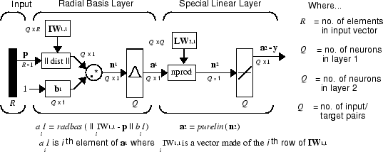
The architecture for the GRNN is shown below. It is similar to the radial basis network, but has a slightly different second layer.

Here the nprod box shown above (code function normprod) produces S² elements in vector n². Each element is the dot product of a row of LW^2,1 and the input vector a¹, all normalized by the sum of the elements of a¹. For instance, suppose that

LW{2,1}= [1 -2;3 4;5 6];
a{1} = [0.7;0.3];

Then

aout = normprod(LW{2,1},a{1})
aout =
    0.1000
    3.3000
    5.3000

The first layer is just like that for newrbe networks. It has as many neurons as there are input/ target vectors in P. Specifically, the first-layer weights are set to P'. The bias b¹ is set to a column vector of 0.8326/SPREAD. The user chooses SPREAD, the distance an input vector must be from a neuron's weight vector to be 0.5.

Again, the first layer operates just like the newrbe radial basis layer described previously. Each neuron's weighted input is the distance between the input vector and its weight vector, calculated with dist. Each neuron's net input is the product of its weighted input with its bias, calculated with netprod. Each neuron's output is its net input passed through radbas. If a neuron's weight vector is equal to the input vector (transposed), its weighted input will be 0, its net input will be 0, and its output will be 1. If a neuron's weight vector is a distance of spread from the input vector, its weighted input will be spread, and its net input will be sqrt(−log(.5)) (or 0.8326). Therefore its output will be 0.5.

The second layer also has as many neurons as input/target vectors, but here LW{2,1} is set to T.

Suppose you have an input vector p close to p_i, one of the input vectors among the input vector/target pairs used in designing layer 1 weights. This input p produces a layer 1 aⁱ output close to 1. This leads to a layer 2 output close to t_i, one of the targets used to form layer 2 weights.

A larger spread leads to a large area around the input vector where layer 1 neurons will respond with significant outputs. Therefore if spread is small the radial basis function is very steep, so that the neuron with the weight vector closest to the input will have a much larger output than other neurons. The network tends to respond with the target vector associated with the nearest design input vector.

As spread becomes larger the radial basis function's slope becomes smoother and several neurons can respond to an input vector. The network then acts as if it is taking a weighted average between target vectors whose design input vectors are closest to the new input vector. As spread becomes larger more and more neurons contribute to the average, with the result that the network function becomes smoother.

Design (newgrnn)

You can use the function newgrnn to create a GRNN. For instance, suppose that three input and three target vectors are defined as

P = [4 5 6];
T = [1.5 3.6 6.7];

You can now obtain a GRNN with

net = newgrnn(P,T);

and simulate it with

P = 4.5;
v = sim(net,P);

You might want to try GRNN Function Approximation as well.