Train Custom Quantile Neural Network

Since R2026a

This example shows how to customize and train a neural network that makes quantile predictions.

In many applications of neural networks, predictions can be uncertain due to noise in the data and inherent randomness in the training algorithm. For example, measurement errors, environmental factors, and other unknown conditions can influence the correct value.

Most neural networks predict a single value given some input data. For example, a neural network might take some sensor readings from a battery unit and predict the battery state of charge. By outputting a single value, the prediction does not capture uncertainty.

A quantile neural network (QNN) is a type of neural network that predicts quantiles. That is, the QNN predicts multiple values that split the possible outcomes into intervals with associated probabilities. For example, given the same sensor readings from a battery unit, a QNN can predict different levels of possible battery states with varying levels of confidence. QNNs are well suited for workflows that involve noisy data or when you want to incorporate elements of risk into your predictions.

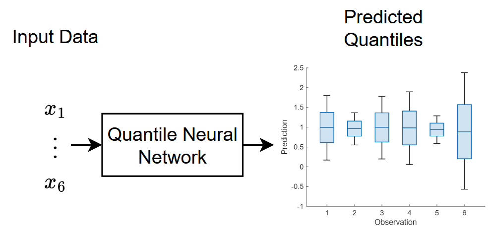
This diagram illustrates the flow of data through a QNN. The neural network predicts various values $μ_{τ}$ where $p (Y \leq μ_{τ} | X) = τ$ , where $τ$ denotes the quantile, $X$ is the network input, and $Y$ is the response variable.

For most tasks, you can use the fitrqnet (Statistics and Machine Learning Toolbox) function to easily train a quantile neural network. For network architectures that do not support the fitrqnet function (such as networks with skip connections or custom weights initializers), or for tasks where you want to customize the training options (for example, further customize the solver options), you can define the neural network as a dlnetwork object and train it using the trainnet function.

This example trains a quantile neural network that has a skip connection and custom weight initializers.

Load Training Data

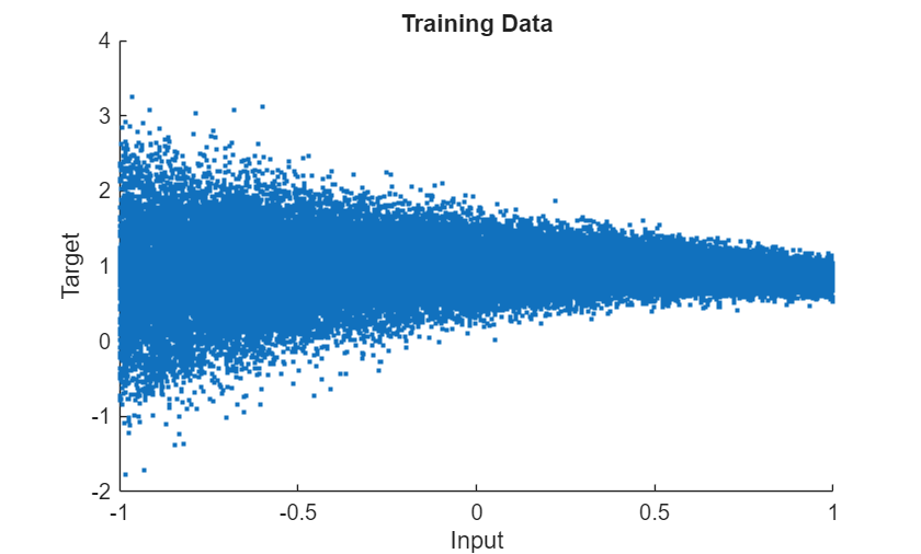
Load the training data. For demonstrative purposes, this example generates a dataset of example inputs and targets. To help demonstrate quantile prediction, the data noise level in the data varies. In general, you do not need to generate data to train a QNN. You can load your own data instead.

Create a function that generates data. For the input data, randomly sample from a uniform distribution with lower and upper bounds of -1 and 1, respectively. For the targets, sample from a normal distribution with mean and standard deviation given by $s i n (x) / x$ and $0.1 e^{1 - x}$ , respectively, where $x$ is the input value.

function [X,T] = generateData(numPoints)

X = 2*rand([numPoints 1]) - 1;

M = sin(X)./X;
Sigma = 0.1*exp(1-X);

T = M + Sigma.*randn(numPoints,1);

end

Generate 50,000 points using the data generation function.

numPoints = 50000;
[X,T] = generateData(numPoints);

Split the data into training, validation, and test partitions using the trainingPartitions function, which is attached to this example as a supporting file. To access this function, open the example as a live script. Use 80% of the data for training, 10% for validation, and the remaining 10% for testing.

[idxTrain,idxValidation,idxTest] = trainingPartitions(numPoints,[0.8 0.1 0.1]);

XTrain = X(idxTrain);
TTrain = T(idxTrain);

XValidation = X(idxValidation);
TValidation = T(idxValidation);

XTest = X(idxTest);
TTest = T(idxTest);

Visualize the training data in a plot.

figure
scatter(X,T,".")
xlabel("Input")
ylabel("Target")
title("Training Data")

Define Neural Network Architecture

Define the quantile neural network architecture.

Use 0.01, 0.25, 0.5, 0.75, and 0.99 for the quantiles. These quantiles represent a broad range of the target distribution. The 0.5 quantile corresponds to the median prediction, while 0.25 and 0.75 represent the interquartile range, capturing the central 50% of the distribution. The 0.01 and 0.99 quantiles provide insight into the extreme lower and upper tails, which is useful for understanding uncertainty and potential outliers in the predictions.
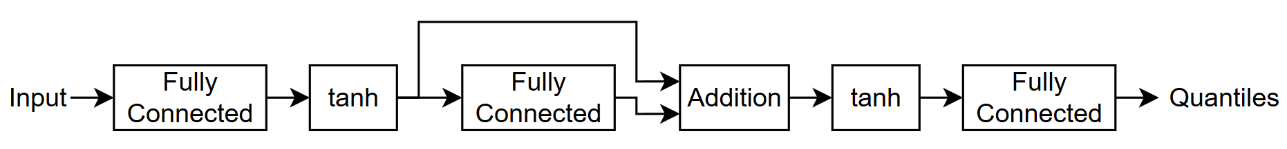
For the input, use a feature input layer with an input size that matches the training data.
Use a simple feedforward network with three fully connected layers with a tanh layer between them.
For the final fully connected layer, specify an output size that matches the number of quantiles.
For the first two fully connected layers, specify an output size of 50.
Add a skip connection around the second fully connected layer. Combine the skip connection with the main branch of the network using an addition layer.
For the fully connected layers, initialize the weights using a normal distribution with a mean of zero and a standard deviation of 0.1.

quantiles = [0.01 0.25 0.5 0.75 0.99];
fcSize = 50;
sig = 0.1;

inputSize = size(XTrain,2);
numQuantiles = numel(quantiles);
initializer = @(sz) sig*randn(sz);

net = dlnetwork;

layers = [
    featureInputLayer(inputSize)
    fullyConnectedLayer(fcSize,WeightsInitializer=initializer)
    tanhLayer(Name="tanh1")
    fullyConnectedLayer(fcSize,WeightsInitializer=initializer)
    additionLayer(2,Name="add")
    tanhLayer
    fullyConnectedLayer(numQuantiles,WeightsInitializer=@(sz) sig*randn(sz))];

net = addLayers(net,layers);
net = connectLayers(net,"tanh1","add/in2");

Define Loss Function

Training a neural network is an optimization task. The task is to find the learnable parameters that minimize a loss function. To train a quantile neural network, you can minimize the quantile loss:

${quantileLoss}_{τ} (Y, T) = {\begin{cases} τ \cdot (T - Y) & if T > Y \\ (1 - τ) \cdot (T - Y) & if T \leq Y \end{cases}$ ,

where $Y$ and $T$ are the predictions and targets, respectively, and $τ$ is the quantile value.

Minimizing the quantile loss ensures that the network predictions for each quantile level match the quantiles of the data. When the predictions and target values are close, the quantile loss is close to zero. The loss function penalizes predictions that are too low for the lower quantiles and predictions that are too high for the upper quantiles.

For batches of data, convert the loss to a scalar value by taking the sum and scaling by the number of observations in the batch.

function loss = quantileLoss(Y,T,quantiles)

quantiles = quantiles(:);

S = T - Y;
L = max(quantiles.*S, (quantiles-1).*S);

N = size(L,2);
loss = sum(L,"all")./N;

end

Specify Training Options

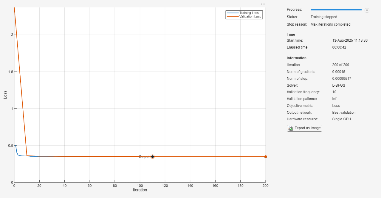
Specify the training options. Choosing among the options requires empirical analysis. To explore different training option configurations by running experiments, you can use the Experiment Manager app.

Train using the L-BFGS solver.
Train for a maximum of 200 iterations.
Validate the network using the validation data every 10 iterations.
Visualize the training progress in a plot.
Disable the verbose output.

options = trainingOptions("lbfgs", ...
    MaxIterations=200, ...
    ValidationData={XValidation,TValidation}, ...
    ValidationFrequency=10, ...
    Plots="training-progress", ...
    Verbose=false);

Train Neural Network

Train the neural network using the trainnet function.

For the QNN, use quantile loss. Because the loss function depends on the $τ$ values, but the trainnet function requires loss functions that take only the predictions and targets as input, specify the loss function as an anonymous function with two inputs only.

By default, the trainnet function uses a GPU if one is available. Using a GPU requires a Parallel Computing Toolbox™ license and a supported GPU device. For information on supported devices, see GPU Computing Requirements (Parallel Computing Toolbox). Otherwise, the function uses the CPU. To select the execution environment manually, use the ExecutionEnvironment training option.

lossFcn = @(Y,T) quantileLoss(Y,T,quantiles);
net = trainnet(XTrain,TTrain,net,lossFcn,options);

Test Neural Network

Test the neural network using the testnet function. Use the same loss function as used for training. A lower value indicates a better fit.

By default, the testnet function uses a GPU if one is available. Otherwise, the function uses the CPU. To select the execution environment manually, use the ExecutionEnvironment argument of the testnet function.

lossTest = testnet(net,XTest,TTest,lossFcn)

lossTest = 
0.3481

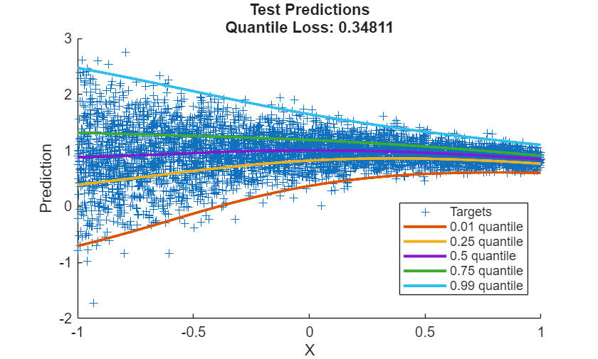
Visualize the test predictions in a plot.

Make predictions using the trained network.

YTest = predict(net,XTest);

For plotting, sort the input values and the corresponding predictions.

[X, idx] = sort(XTest);
Y = YTest(idx,:);

Display the targets using a scatter plot.

figure
scatter(XTest,TTest,"+",DisplayName="Targets")

Add the predicted quantiles to the scatter plot. For each quantile, plot a line with width 2.

hold on

for i = 1:numQuantiles
    plot(X,Y(:,i), ...
        DisplayName=quantiles(i) + " quantile", ...
        LineWidth=2)
end

xlabel("X")
ylabel("Prediction")

hold off
legend(Location="Best")
title( ...
    "Test Predictions" + newline ...
    + "Quantile Loss: " + lossTest)

Make Predictions With New Data

Select some input values to make predictions with.

numObservationsNew = 6;
XNew = 2*rand([numObservationsNew 1]) - 1

Predict the quantiles using the predict function.

YNew = predict(net,XNew);

Visualize the predicted quantiles using a box chart. In this example, each box spans from the lower to upper quantiles (the 0.25 and 0.75 quantiles, respectively), and indicates the median (the 0.5 quantile) as the center of the box.

figure
boxchart(YNew')
xlabel("Observation")
ylabel("Prediction")
title("Predicted Quantiles")

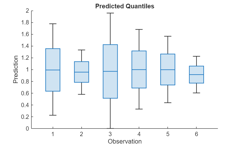
This plot shows a visual summary of the model's predictive uncertainty and the range of possible outcomes for each input. Narrower boxes indicate higher confidence in the predictions, while wider boxes indicate greater uncertainty.