trainingOptions
Options for training deep learning neural network
Description
options = trainingOptions(solverName)solverName. To train a neural network, use the
training options as an input argument to the trainnet function.
options = trainingOptions(solverName,Name=Value)
Examples
Create a set of options for training a network using stochastic gradient descent with momentum. Reduce the learning rate by a factor of 0.2 every 5 epochs. Set the maximum number of epochs for training to 20, and use a mini-batch with 64 observations at each iteration. Turn on the training progress plot.
options = trainingOptions("sgdm", ...
    LearnRateSchedule="piecewise", ...
    LearnRateDropFactor=0.2, ...
    LearnRateDropPeriod=5, ...
    MaxEpochs=20, ...
    MiniBatchSize=64, ...
    Plots="training-progress")
options =
  TrainingOptionsSGDM with properties:

                        Momentum: 0.9000
                       MaxEpochs: 20
                InitialLearnRate: 0.0100
               LearnRateSchedule: 'piecewise'
             LearnRateDropFactor: 0.2000
             LearnRateDropPeriod: 5
                   MiniBatchSize: 64
                         Shuffle: 'once'
         CheckpointFrequencyUnit: 'epoch'
        PreprocessingEnvironment: 'serial'
                         Verbose: 1
                VerboseFrequency: 50
                  ValidationData: []
             ValidationFrequency: 50
              ValidationPatience: Inf
                         Metrics: []
             ObjectiveMetricName: 'loss'
            ExecutionEnvironment: 'auto'
                           Plots: 'training-progress'
                       OutputFcn: []
                  SequenceLength: 'longest'
            SequencePaddingValue: 0
        SequencePaddingDirection: 'right'
                InputDataFormats: "auto"
               TargetDataFormats: "auto"
         ResetInputNormalization: 1
       ResetInverseNormalization: 1
                NormalizeTargets: 0
    BatchNormalizationStatistics: 'auto'
                   OutputNetwork: 'auto'
                    Acceleration: "auto"
                  CheckpointPath: ''
             CheckpointFrequency: 1
        CategoricalInputEncoding: 'integer'
       CategoricalTargetEncoding: 'auto'
                L2Regularization: 1.0000e-04
         GradientThresholdMethod: 'l2norm'
               GradientThreshold: Inf
This example shows how to monitor the training progress of deep learning networks.
When you train networks for deep learning, plotting various metrics during training enables you to learn how the training is progressing. For example, you can determine if and how quickly the network accuracy is improving, and whether the network is starting to overfit the training data.
This example shows how to monitor training progress for networks trained using the trainnet function. If you are training a network using a custom training loop, use a trainingProgressMonitor object instead to plot metrics during training. For more information, see Monitor Custom Training Loop Progress.
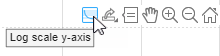
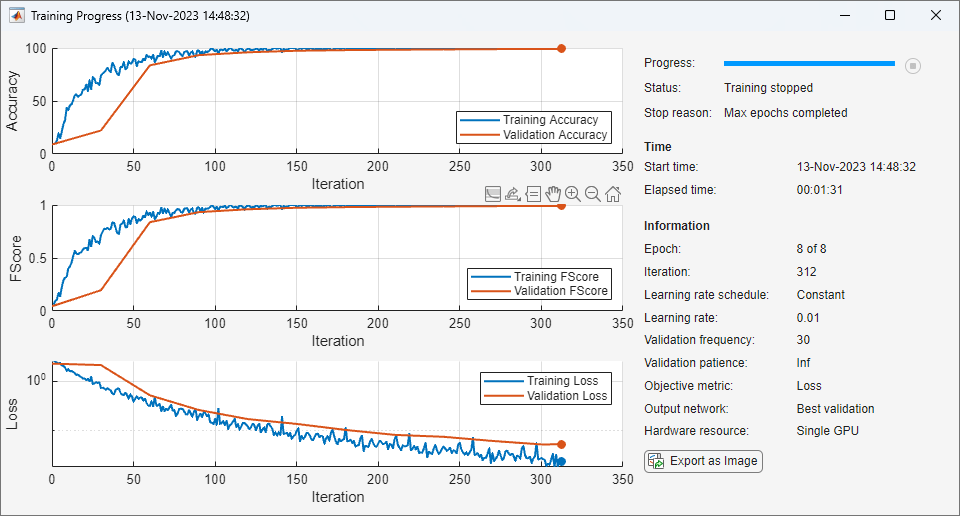
When you set the Plots training option to "training-progress" in trainingOptions and start network training, the trainnet function creates a figure and displays training metrics at every iteration. Each iteration is an estimation of the gradient and an update of the network parameters. If you specify validation data in trainingOptions, then the figure shows validation metrics each time trainnet validates the network. The figure plots the loss and any metrics specified by the Metrics name-value option. By default, the software uses a linear scale for the plots. To specify a logarithmic scale for the y-axis, select the log scale button in the axes toolbar.
During training, you can stop training and return the current state of the network by clicking the stop button in the top-right corner. After you click the stop button, it can take a while for training to complete. Once training is complete, trainnet returns the trained network.
Specify the OutputNetwork training option as "best-validation" to get finalized values that correspond to the iteration with the best validation metric value, where the optimized metric is specified by the ObjectiveMetricName training options. Specify the OutputNetwork training option as "last-iteration" to get finalized metrics that correspond to the last training iteration.
On the right of the pane, view information about the training time and settings. To learn more about training options, see Set Up Parameters and Train Convolutional Neural Network.
To save the training progress plot, click Export as Image in the training window. You can save the plot as a PNG, JPEG, TIFF, or PDF file. You can also save the individual plots using the axes toolbar.
Plot Training Progress During Training
Train a network and plot the training progress during training.
Load the training and test data from the MAT files DigitsDataTrain.mat and DigitsDataTest.mat, respectively. The training and test data sets each contain 5000 images.
load DigitsDataTrain.mat
load DigitsDataTest.mat
Create a dlnetwork object.
net = dlnetwork;
Specify the layers of the classification branch and add them to the network.
layers = [
    imageInputLayer([28 28 1])
    convolution2dLayer(3,8,Padding="same")
    batchNormalizationLayer
    reluLayer
    maxPooling2dLayer(2,Stride=2)
    convolution2dLayer(3,16,Padding="same")
    batchNormalizationLayer
    reluLayer
    maxPooling2dLayer(2,Stride=2)
    convolution2dLayer(3,32,Padding="same")
    batchNormalizationLayer
    reluLayer
    fullyConnectedLayer(10)
    softmaxLayer];

net = addLayers(net,layers);
Specify options for network training. To validate the network at regular intervals during training, specify validation data. Record the metric values for the accuracy and F-score. To plot training progress during training, set the Plots training option to "training-progress".
options = trainingOptions("sgdm", ...
    MaxEpochs=8, ...
    Metrics = ["accuracy","fscore"], ...
    ValidationData={XTest,labelsTest}, ...
    ValidationFrequency=30, ...
    Verbose=false, ...
    Plots="training-progress");
Train the network.
net = trainnet(XTrain,labelsTrain,net,"crossentropy",options);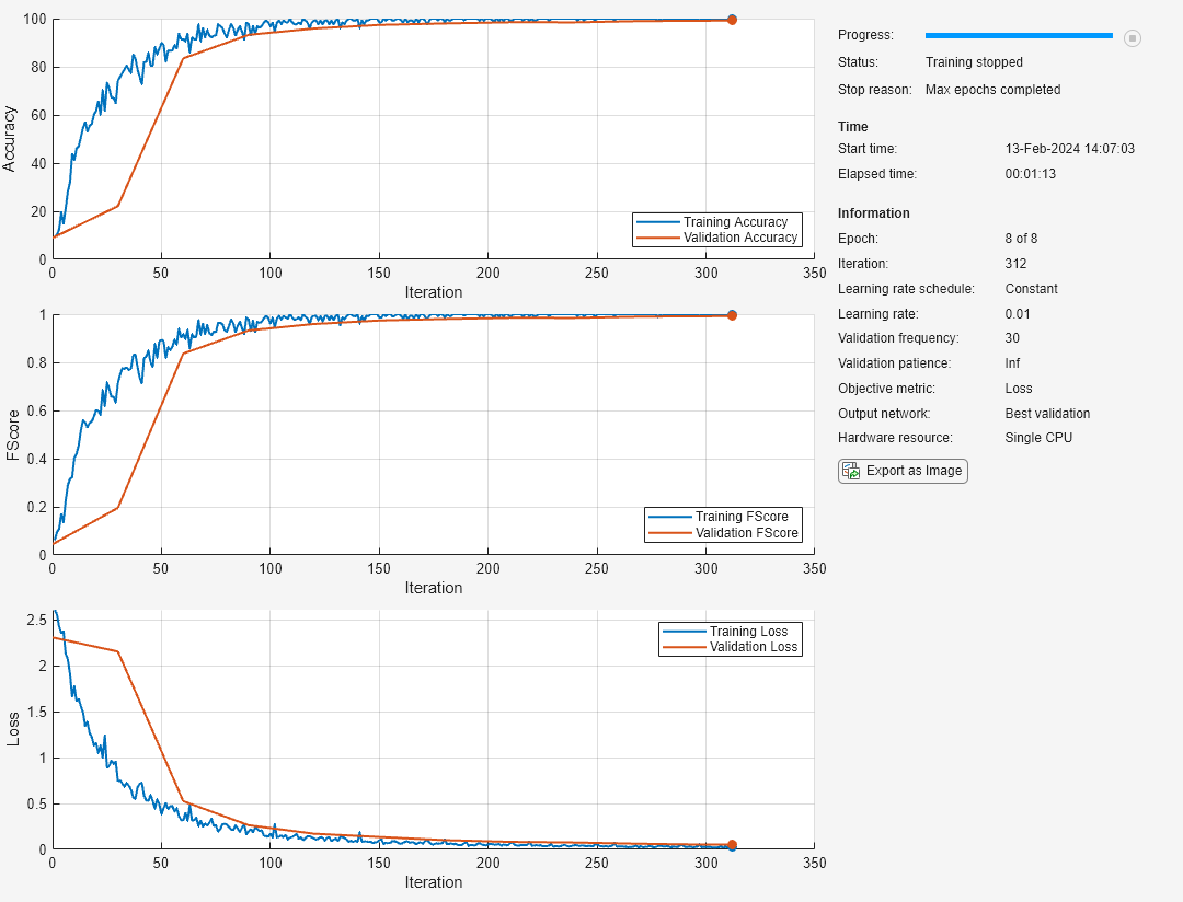
Use metrics for early stopping and to return the best network.
Load the training data, which contains 5000 images of digits. Set aside 1000 of the images for network validation.
[XTrain,YTrain] = digitTrain4DArrayData;

idx = randperm(size(XTrain,4),1000);
XValidation = XTrain(:,:,:,idx);
XTrain(:,:,:,idx) = [];
YValidation = YTrain(idx);
YTrain(idx) = [];
Construct a network to classify the digit image data.
net = dlnetwork;

layers = [
    imageInputLayer([28 28 1])
    convolution2dLayer(3,8,Padding="same")
    batchNormalizationLayer
    reluLayer
    fullyConnectedLayer(10)
    softmaxLayer];

net = addLayers(net,layers);
Specify the training options:
Use an SGDM solver for training.
Monitor training performance by specifying validation data and validation frequency.
Track the accuracy and recall during training. To return the network with the best recall value, specify
"recall"as the objective metric and set the output network to"best-validation".Specify the validation patience as 5 so training stops if the recall has not decreased for five iterations.
Visualize network training progress plot.
Suppress the verbose output.
options = trainingOptions("sgdm", ...
    ValidationData={XValidation,YValidation}, ...
    ValidationFrequency=35, ...
    ValidationPatience=5, ...
    Metrics=["accuracy","recall"], ...
    ObjectiveMetricName="recall", ...
    OutputNetwork="best-validation", ...
    Plots="training-progress", ...
    Verbose=false);
Train the network.
net = trainnet(XTrain,YTrain,net,"crossentropy",options);
Input Arguments
Name-Value Arguments
Specify optional pairs of arguments as
Name1=Value1,...,NameN=ValueN, where Name is
the argument name and Value is the corresponding value.
Name-value arguments must appear after other arguments, but the order of the
pairs does not matter.
Before R2021a, use commas to separate each name and value, and enclose
Name in quotes.
Example: Plots="training-progress",Metrics="accuracy",Verbose=false
specifies to disable the verbose output and display the training progress in
a plot that also includes the accuracy metric.
Monitoring
Plots to display during neural network training, specified as one of these values:
"none"— Do not display plots during training."training-progress"— Plot training progress.
The contents of the plot depends on the solver that you use.
When the
solverNameargument is"sgdm","adam", or"rmsprop", the plot shows the mini-batch loss, validation loss, training mini-batch and validation metrics specified by theMetricsoption, and additional information about the training progress.When the
solverNameargument is"lbfgs"or"lm", the plot shows the training and validation loss, training and validation metrics specified by theMetricsoption, and additional information about the training progress.
To programmatically open and close the training progress plot after training, use the show and close functions with the second output of the trainnet function. You can use the show function to view the training progress even if the Plots training option is specified as "none".
To switch the y-axis scale to logarithmic, use the axes toolbar. 
For more information about the plot, see Monitor Deep Learning Training Progress.
Since R2023b
Metrics to monitor, specified as one of these values:
Built-in metric or loss function name — Specify metrics as a string scalar, character vector, cell array, or string array of one or more of these names:
Metrics:
"accuracy"— Accuracy (also known as top-1 accuracy)"auc"— Area under ROC curve (AUC)"fscore"— F-score (also known as F1-score)"precision"— Precision"recall"— Recall"rmse"— Root mean squared error"mape"— Mean absolute percentage error (MAPE) (since R2024b)"rsquared"— R2 (R-squared or coefficient of determination) (since R2025a)
Loss functions:
"crossentropy"— Cross-entropy loss for classification tasks (since R2024b)"indexcrossentropy"— Index cross-entropy loss for classification tasks (since R2024b)"binary-crossentropy"— Binary cross-entropy loss for binary and multilabel classification tasks (since R2024b)"mae"/"mean-absolute-error"/"l1loss"— Mean absolute error for regression tasks (since R2024b)"mse"/"mean-squared-error"/"l2loss"— Mean squared error for regression tasks (since R2024b)"huber"— Huber loss for regression tasks (since R2024b)
Setting the loss function as
"crossentropy"and specifying"index-crossentropy"as a metric or setting the loss function as"index-crossentropy"and specifying"crossentropy"as a metric is not supported.For more information about deep learning metrics and loss functions, see Deep Learning Metrics.
Built-in metric objects — If you need more flexibility, you can use built-in metric objects. The software supports these built-in metric objects:
MAPEMetric(since R2024b)RSquaredMetric(since R2025a)
When you create a built-in metric object, you can specify additional options such as the averaging type and whether the task is single-label or multilabel.
Custom metric function handle — If the metric you need is not a built-in metric, then you can specify custom metrics using a function handle. The function must have the syntax
metric = metricFunction(Y,T), whereYcorresponds to the network predictions andTcorresponds to the target responses. For networks with multiple outputs, the syntax must bemetric = metricFunction(Y1,...,YN,T1,...,TM), whereNis the number of outputs andMis the number of targets. For more information, see Define Custom Metric Function.Note
When you have data in mini-batches, the software computes the metric for each mini-batch and then returns the average of those values. For some metrics, this behavior can result in a different metric value than if you compute the metric using the whole data set at once. In most cases, the values are similar. To use a custom metric that is not batch-averaged for the data, you must create a custom metric object. For more information, see Define Custom Deep Learning Metric Object.
deep.DifferentiableFunctionobject (since R2024a) — Function object with custom backward function. For categorical targets, the software automatically converts the categorical values to one-hot encoded vectors and passes them to the metric function. For more information, see Define Custom Deep Learning Operations.Custom metric object — If you need greater customization, then you can define your own custom metric object. For an example that shows how to create a custom metric, see Define Custom Metric Object. For general information about creating custom metrics, see Define Custom Deep Learning Metric Object.
If you specify a metric as a function handle, a deep.DifferentiableFunction
object, or a custom metric object and train the neural network using the
trainnet function, then the layout of the targets that the software
passes to the metric depends on the data type of the targets. The loss function that you
specify in the trainnet function and the other metrics that you specify
have these effects on the software:
If the targets are numeric arrays, then the software passes the targets to the metric directly.
If the loss function is
"index-crossentropy"and the targets are categorical arrays, then the software automatically converts the targets to numeric class indices and passes them to the metric.For other loss functions, if the targets are categorical arrays, then the software automatically converts the targets to one-hot encoded vectors and then passes them to the metric.
This option supports the trainnet and
trainBERTDocumentClassifier (Text Analytics Toolbox) functions only.
Example: Metrics=["accuracy","fscore"]
Example: Metrics={"accuracy",@myFunction,precisionObj}
Since R2024a
Name of objective metric to use for early stopping and returning the best network, specified as a string scalar or character vector.
The metric name must be "loss" or match the name of a metric specified by
the Metrics argument. Metrics specified using function handles are not
supported. To specify the ObjectiveMetricName value as the name of a
custom metric, the value of the Maximize property of the custom metric
object must be nonempty. For more information, see Define Custom Deep Learning Metric Object.
For more information about specifying the objective metric for early stopping, see ValidationPatience. For more information about returning the best network using the objective metric, see OutputNetwork.
Data Types: char | string
Flag to display training progress information in the
command window, specified as 1
(true) or 0
(false).
The content of the verbose output depends on the type of solver.
For stochastic solvers (SGDM, Adam, and RMSProp), the table contains these variables:
| Variable | Description |
|---|---|
Iteration | Iteration number. |
Epoch | Epoch number. |
TimeElapsed | Time elapsed in hours, minutes, and seconds. |
LearnRate | Learning rate. |
TrainingLoss | Training loss. |
ValidationLoss | Validation loss. If you do not specify validation data, then the software does not display this information. |
For batch solvers (L-BFGS and LM), the table contains these variables:
| Variable | Description |
|---|---|
Iteration | Iteration number |
TimeElapsed | Time elapsed in hours, minutes, and seconds |
TrainingLoss | Training loss |
ValidationLoss | Validation loss. If you do not specify validation data, then the software does not display this information. |
GradientNorm | Norm of the gradients |
StepNorm | Norm of the steps |
If you specify additional metrics in the training options, then
they also appear in the verbose output. For example, if you set the Metrics
training option to "accuracy", then the information includes the
TrainingAccuracy and ValidationAccuracy
variables.
When training stops, the verbose output displays the reason for stopping.
To specify validation data, use the ValidationData training option.
Data Types: single | double | int8 | int16 | int32 | int64 | uint8 | uint16 | uint32 | uint64 | logical
Frequency of verbose printing, which is the number of iterations between printing to the Command Window, specified as a positive integer.
If you validate the neural network during training, then the software also prints to the Command Window every time validation occurs.
To enable this property, set the Verbose training option to
1 (true).
Data Types: single | double | int8 | int16 | int32 | int64 | uint8 | uint16 | uint32 | uint64
Output functions to call during training, specified as a function handle or cell array of function handles. The software calls the functions once before the start of training, after each iteration, and once when training is complete.
The functions must have the syntax stopFlag = f(info), where info is a structure containing information about the training progress, and stopFlag is a scalar that indicates to stop training early. If stopFlag is 1 (true), then the software stops training. Otherwise, the software continues training.
The trainnet function passes the
output function the structure info.
For stochastic solvers (SGDM, Adam, and RMSProp),
info contains these fields:
| Field | Description |
|---|---|
Epoch | Epoch number |
Iteration | Iteration number |
TimeElapsed | Time since start of training |
LearnRate | Iteration learn rate |
TrainingLoss | Iteration training loss |
ValidationLoss | Validation loss, if specified and evaluated at iteration. |
State | Iteration training state, specified as "start", "iteration", or "done". |
For batch solvers (L-BFGS and LM), info
contains these fields:
| Field | Description |
|---|---|
Iteration | Iteration number |
TimeElapsed | Time elapsed in hours, minutes, and seconds |
TrainingLoss | Training loss |
ValidationLoss | Validation loss. If you do not specify validation data, then the software does not display this information. |
GradientNorm | Norm of the gradients |
StepNorm | Norm of the steps |
State | Iteration training state, specified as "start",
"iteration", or "done" |
If you specify additional metrics in the training options, then
they also appear in the training information. For example, if you set the
Metrics training option to "accuracy", then the
information includes the TrainingAccuracy and
ValidationAccuracy fields.
If a field is not calculated or relevant for a certain call to the output functions, then that field contains an empty array.
For an example showing how to use output functions, see Custom Stopping Criteria for Deep Learning Training.
Data Types: function_handle | cell
Data Layout
Stochastic Solver Options
Maximum number of epochs (full passes of the data) to use for training, specified as a positive integer.
This option supports stochastic solvers only (when the solverName
argument is "sgdm", "adam", or
"rmsprop").
Data Types: single | double | int8 | int16 | int32 | int64 | uint8 | uint16 | uint32 | uint64
Size of the mini-batch to use for each training iteration, specified as a positive integer. A mini-batch is a subset of the training set that is used to evaluate the gradient of the loss function and update the weights.
If the mini-batch size does not evenly divide the number of training samples, then the software discards the training data that does not fit into the final complete mini-batch of each epoch. If the mini-batch size is smaller than the number of training samples, then the software does not discard any data.
This option supports stochastic solvers only (when the solverName
argument is "sgdm", "adam", or
"rmsprop").
Tip
For best performance, if you are training a network using a datastore with a
ReadSize property, such as an imageDatastore, then set the ReadSize property and
MiniBatchSize training option to the same value. If you are
training a network using a datastore with a MiniBatchSize property,
such as an augmentedImageDatastore, then set the MiniBatchSize
property of the datastore and the MiniBatchSize training option to the
same value.
Data Types: single | double | int8 | int16 | int32 | int64 | uint8 | uint16 | uint32 | uint64
Option for data shuffling, specified as one of these values:
"once"— Shuffle the training and validation data once before training."never"— Do not shuffle the data."every-epoch"— Shuffle the training data before each training epoch, and shuffle the validation data before each neural network validation. If the mini-batch size does not evenly divide the number of training samples, then the software discards the training data that does not fit into the final complete mini-batch of each epoch. To avoid discarding the same data every epoch, set theShuffletraining option to"every-epoch".
This option supports stochastic solvers only (when the solverName
argument is "sgdm", "adam", or
"rmsprop").
Initial learning rate used for training, specified as a positive scalar.
If the learning rate is too low, then training can take a long time. If the learning rate is too high, then training might reach a suboptimal result or diverge.
This option supports stochastic solvers only (when the solverName
argument is "sgdm", "adam", or
"rmsprop").
When solverName is
"sgdm", the default value is
0.01. When
solverName is
"rmsprop" or
"adam", the default value is
0.001.
Data Types: single | double | int8 | int16 | int32 | int64 | uint8 | uint16 | uint32 | uint64
Learning rate schedule, specified as a character vector or string scalar of a built-in learning rate schedule name, a string array of names, a built-in or custom learning rate schedule object, a function handle, or a cell array of names, metric objects, and function handles.
This option supports stochastic solvers only (when the solverName
argument is "sgdm", "adam", or
"rmsprop").
Built-In Learning Rate Schedule Names
Specify learning rate schedules as a string scalar, character vector, or a string or cell array of one or more of these names:
| Name | Description | Plot |
|---|---|---|
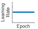
"none" | No learning rate schedule. This schedule keeps the learning rate constant. |
|
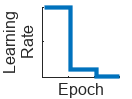
"piecewise" | Piecewise learning rate schedule. Every 10 epochs, this schedule drops the learn rate by a factor of 10. |
|
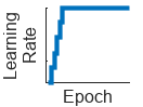
"warmup" (since R2024b) | Warm-up learning rate schedule. For 5 iterations, this schedule ramps up the learning rate to the base learning rate. |
|
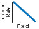
"polynomial" (since R2024b) | Polynomial learning rate schedule. Every epoch, this schedule drops the learning rate using a power law with a unitary exponent. |
|
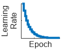
"exponential" (since R2024b) | Exponential learning rate schedule. Every epoch, this schedule decays
the learning rate by a factor of 10. |
|
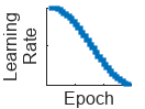
"cosine" (since R2024b) | Cosine learning rate schedule. Every epoch, this schedule drops the learn rate using a cosine formula. |
|
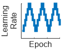
"cyclical" (since R2024b) | Cyclical learning rate schedule. For periods of 10 epochs, this schedule increases the learning rate from the base learning rate for 5 epochs and then decreases the learning rate for 5 epochs. |
|
Built-In Learning Rate Schedule Object (since R2024b)
If you need more flexibility than what the string options provide, you can use built-in learning rate schedule objects:
piecewiseLearnRate— A piecewise learning rate schedule object drops the learning rate periodically by multiplying it by a specified factor. Use this object to customize the drop factor and period of the piecewise schedule.Before R2024b: Customize the piecewise drop factor and period using the
LearnRateDropFactorandLearnRateDropPeriodtraining options, respectively.warmupLearnRate— A warm-up learning rate schedule object ramps up the learning for a specified number of iterations. Use this object to customize the initial and final learning rate factors and the number of steps of the warm up schedule.polynomialLearnRate— A polynomial learning rate schedule drops the learning rate using a power law. Use this object to customize the initial and final learning rate factors, the exponent, and the number of steps of the polynomial schedule.exponentialLearnRate— An exponential learning rate schedule decays the learning rate by a specified factor. Use this object to customize the drop factor and period of the exponential schedule.cosineLearnRate— A cosine learning rate schedule object drops the learning rate using a cosine curve and incorporates warm restarts. Use this object to customize the initial and final learning rate factors, the period, and the period growth factor of the cosine schedule.cyclicalLearnRate— A cyclical learning rate schedule periodically increases and decreases the learning rate. Use this option to customize the maximum factor, period, and step ratio of the cyclical schedule.
Custom Learning Rate Schedule (since R2024b)
For additional flexibility, you can define a custom learning rate schedule as a function handle or custom class that inherits from deep.LearnRateSchedule.
Custom learning rate schedule function handle — If the learning rate schedule you need is not a built-in learning rate schedule, then you can specify custom learning rate schedules using a function handle. To specify a custom schedule, use a function handle with the syntax
learningRate =
                        f(baseLearningRate,epoch)
, wherebaseLearningRateis the base learning rate, andepochis the epoch number.Custom learn rate schedule object — If you need more flexibility that what function handles provide, then you can define a custom learning rate schedule class that inherits from
deep.LearnRateSchedule.
Multiple Learning Rate Schedules (since R2024b)
You can combine multiple learning rate schedules by specifying multiple schedules as a string
or cell array and then the software applies the schedules in order, starting with the first
element. At most one of the schedules can be infinite (schedules than continue indefinitely,
such as "cyclical" and objects with the NumSteps
property set to Inf) and the infinite schedule must be the last element
of the array.
Contribution of the parameter update step of the previous iteration to the current iteration of stochastic gradient descent with momentum, specified as a scalar from 0 to 1.
A value of 0 means no contribution from the previous step, whereas a value of 1 means maximal contribution from the previous step. The default value works well for most tasks.
This argument supports the SGDM solver only (when the
solverName argument is
"sgdm").
For more information, see Stochastic Gradient Descent with Momentum.
Data Types: single | double | int8 | int16 | int32 | int64 | uint8 | uint16 | uint32 | uint64
Decay rate of gradient moving average for the Adam solver, specified as a nonnegative scalar less than 1. The gradient decay rate is denoted by β1 in the Adaptive Moment Estimation section.
This argument supports the Adam solver only (when the
solverName argument is
"adam").
For more information, see Adaptive Moment Estimation.
Data Types: single | double | int8 | int16 | int32 | int64 | uint8 | uint16 | uint32 | uint64
Decay rate of squared gradient moving average for the Adam
and RMSProp solvers, specified as a nonnegative scalar
less than 1. The squared gradient decay
rate is denoted by
β2 in
[4].
Typical values of the decay rate are 0.9, 0.99, and 0.999, corresponding to averaging lengths of 10, 100, and 1000 parameter updates, respectively.
This option supports the Adam and RMSProp solvers only (when the solverName argument is "adam" or
"rmsprop").
The default value is 0.999 for the Adam
solver. The default value is 0.9 for
the RMSProp solver.
For more information, see Adaptive Moment Estimation and Root Mean Square Propagation.
Data Types: single | double | int8 | int16 | int32 | int64 | uint8 | uint16 | uint32 | uint64
Denominator offset for Adam and RMSProp solvers, specified as a positive scalar.
The solver adds the offset to the denominator in the neural network parameter updates to avoid division by zero. The default value works well for most tasks.
This option supports the Adam and RMSProp solvers only (when the solverName argument is "adam" or
"rmsprop").
For more information, see Adaptive Moment Estimation and Root Mean Square Propagation.
Data Types: single | double | int8 | int16 | int32 | int64 | uint8 | uint16 | uint32 | uint64
Factor for dropping the learning rate, specified as a scalar from 0 to
1. This argument is valid only when the
LearnRateSchedule argument is
"piecewise".
LearnRateDropFactor is a multiplicative factor to apply to the learning
rate every time a certain number of epochs passes. Specify the number of epochs using the
LearnRateDropPeriod argument.
This option supports stochastic solvers only (when the solverName
argument is "sgdm", "adam", or
"rmsprop").
Tip
To customize the piecewise learning rate schedule, use a piecewiseLearnRate object. A piecewiseLearnRate object is recommended over the LearnRateDropFactor and LearnRateDropPeriod training options because it provides additional control over the drop frequency. (since R2024b)
Data Types: single | double | int8 | int16 | int32 | int64 | uint8 | uint16 | uint32 | uint64
Number of epochs for dropping the learning rate, specified as a positive integer. This
argument is valid only when the LearnRateSchedule value is
"piecewise".
The software multiplies the global learning rate with the drop factor every time the specified
number of epochs passes. Specify the drop factor using the
LearnRateDropFactor argument.
This option supports stochastic solvers only (when the solverName
argument is "sgdm", "adam", or
"rmsprop").
Tip
To customize the piecewise learning rate schedule, use a piecewiseLearnRate object. A piecewiseLearnRate object is recommended over the LearnRateDropFactor and LearnRateDropPeriod training options because it provides additional control over the drop frequency. (since R2024b)
Data Types: single | double | int8 | int16 | int32 | int64 | uint8 | uint16 | uint32 | uint64
Batch Solver Options
Validation
Normalization and Regularization
Gradient Clipping
Sequence
Hardware and Acceleration
Checkpoints
Output Arguments
Tips
For most deep learning tasks, you can use a pretrained neural network and adapt it to your own data. For an example showing how to use transfer learning to retrain a convolutional neural network to classify a new set of images, see Retrain Neural Network to Classify New Images. Alternatively, you can create and train neural networks from scratch using the
trainnetandtrainingOptionsfunctions.If the
trainingOptionsfunction does not provide the training options that you need for your task, then you can create a custom training loop using automatic differentiation. To learn more, see Train Network Using Custom Training Loop.If the
trainnetfunction does not provide the loss function that you need for your task, then you can specify a custom loss function to thetrainnetas a function handle. For loss functions that require more inputs than the predictions and targets (for example, loss functions that require access to the neural network or additional inputs), train the model using a custom training loop. To learn more, see Train Network Using Custom Training Loop.If Deep Learning Toolbox™ does not provide the layers you need for your task, then you can create a custom layer. To learn more, see Define Custom Deep Learning Layers. For models that cannot be specified as networks of layers, you can define the model as a function. To learn more, see Train Network Using Model Function.
For more information about which training method to use for which task, see Train Deep Learning Model in MATLAB.
Algorithms
References
[1] Bishop, C. M. Pattern Recognition and Machine Learning. Springer, New York, NY, 2006.
[2] Murphy, K. P. Machine Learning: A Probabilistic Perspective. The MIT Press, Cambridge, Massachusetts, 2012.
[3] Pascanu, R., T. Mikolov, and Y. Bengio. "On the difficulty of training recurrent neural networks". Proceedings of the 30th International Conference on Machine Learning. Vol. 28(3), 2013, pp. 1310–1318.
[4] Kingma, Diederik, and Jimmy Ba. "Adam: A method for stochastic optimization." arXiv preprint arXiv:1412.6980 (2014).
[5] Liu, Dong C., and Jorge Nocedal. "On the limited memory BFGS method for large scale optimization." Mathematical programming 45, no. 1 (August 1989): 503-528. https://doi.org/10.1007/BF01589116.
[6] Marquardt, Donald W. “An Algorithm for Least-Squares Estimation of Nonlinear Parameters.” Journal of the Society for Industrial and Applied Mathematics 11, no. 2 (June 1963): 431–41. https://doi.org/10.1137/0111030.
Version History
Introduced in R2016aSee Also
trainnet | dlnetwork | analyzeNetwork | Deep Network
Designer