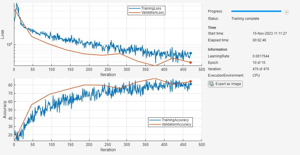
Monitor Custom Training Loop Progress

When you train networks for deep learning, it is often useful to monitor the training progress. By plotting various metrics during training, you can learn how the training is progressing. For example, you can determine whether and how quickly the network accuracy is improving, and whether the network is starting to overfit the training data.

To monitor and plot the training progress of a custom training loop, use a TrainingProgressMonitor object. You can use a TrainingProgressMonitor to:

Create animated custom metric plots and record custom metrics during training.
Display and record training information during training.
Stop training early.
Track training progress with a progress bar.
Track elapsed time.

If you are training a network using the trainnet function and the Plots training option is "training-progress", then the software automatically plots metrics during training. For more information, see Monitor Deep Learning Training Progress.

Create Training Progress Monitor

Create a custom training progress monitor using the trainingProgressMonitor function.

monitor = trainingProgressMonitor;

The TrainingProgressMonitor object automatically tracks elapsed time. The timer starts when you create the TrainingProgressMonitor object. To ensure that the elapsed time accurately reflects the training time, create the monitor object immediately before the start of your training loop.

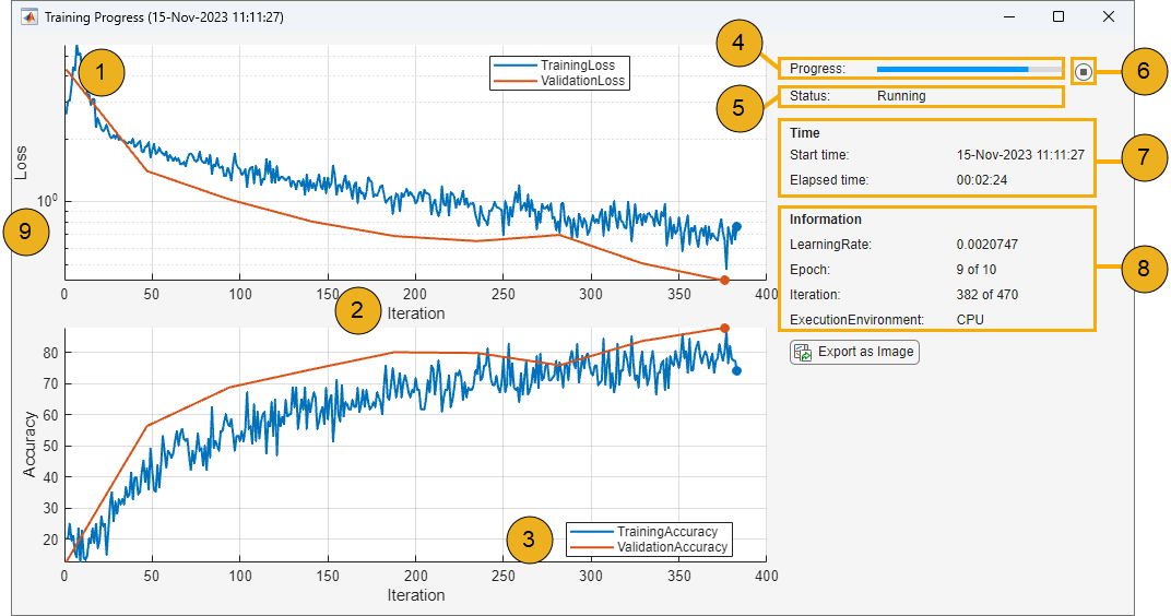
Training Progress Window

Control the display of the Training Progress window using the properties of the TrainingProgressMonitor object. You can set the properties before, during, or after training. For an example showing how to use the monitor to track training progress, see Monitor Custom Training Loop Progress During Training.


monitor.Metrics = ["TrainingLoss","ValidationLoss"];
recordMetrics(monitor,iteration, ...
TrainingLoss=lossTrain, ...
ValidationLoss=lossValidation);
monitor.XLabel = "Iteration";
groupSubPlot(monitor, ...
    "Accuracy",["TrainingAccuracy","ValidationAccuracy"]);
monitor.Progress = 100*(currentIteration/maxIterations);
monitor.Status = "Running";
while numEpochs < maxEpochs && ~monitor.Stop    
% Custom training loop code.   
end
monitor = trainingProgressMonitor;
monitor.Info = ["Epoch","LearningRate"];
updateInfo(monitor, ...
Epoch=currentEpoch, ...
LearningRate=learnRate);
yscale(monitor,"Loss","log")

Example Training Progress Window	Key	Properties and Settings	Example Code
For an example showing how to generate this figure, see Monitor Custom Training Loop Progress During Training.	1	Specify metrics to plot using the `Metrics` property.	Add metric names before training. monitor.Metrics = ["TrainingLoss","ValidationLoss"];
Add new points to the plot and save the values in the `MetricValues` property using `recordMetrics`. The `recordMetrics` function requires metric values and the training loop step, such as an iteration or epoch. In the training plots, the metric values correspond to the y-coordinate and the training loop step corresponds to the x-coordinate.	Update metric values during training. recordMetrics(monitor,iteration, ... TrainingLoss=lossTrain, ... ValidationLoss=lossValidation);
2	Set the x-axis label using the `XLabel` property.	Set the x-axis label to `Iteration`. monitor.XLabel = "Iteration";
3	Group metrics into a single training subplot using the `groupSubPlot` function.	Group the training and validation accuracy plots. groupSubPlot(monitor, ... "Accuracy",["TrainingAccuracy","ValidationAccuracy"]);
4	Track training progress using the `Progress` property. The progress value must be a number in the range [0,100]. This value appears as a progress bar in the Training Progress window.	Set the training progress percentage. monitor.Progress = 100*(currentIteration/maxIterations);
5	Track training status by setting the `Status` property.	Set the current status to `"Running"`. monitor.Status = "Running";
6	Enable early stopping. When you click the Stop button, the `Stop` property changes to `1` (`true`). The training stops if your training loop exits when the `Stop` property is `1`.	To enable early stopping, include the following code in your custom training loop. while numEpochs < maxEpochs && ~monitor.Stop % Custom training loop code. end
7	Track the start and elapsed time. Timing starts when you create the `TrainingProgressMonitor` object.	Create a monitor and start the timer. monitor = trainingProgressMonitor;
8	Display information in the Training Progress window using the `Info` property. The information values are displayed in the Training Progress window but do not appear in plots. Use information for text and numerical values that you want to display in the Training Progress window.	Add information names before training. monitor.Info = ["Epoch","LearningRate"];
Update information values in the Training Progress window and save the values in the `InfoData` property using the `updateInfo` function.	Update information values during training. updateInfo(monitor, ... Epoch=currentEpoch, ... LearningRate=learnRate);
9	Specify the y-axis scale using the `yscale` function. You can also change the scale by clicking the log scale button in the axes toolbar.	Set the loss plot scale to logarithmic. yscale(monitor,"Loss","log")

Monitor Custom Training Loop Progress During Training

Open Live Script

This example shows how to monitor the progress of a deep learning custom training loop.

Load Training Data

Unzip the digit sample data and create an image datastore. The imageDatastore function automatically labels the images based on folder names.

unzip("DigitsData.zip")

imds = imageDatastore("DigitsData", ...
    IncludeSubfolders=true, ...
    LabelSource="foldernames");

Partition the data into training and validation sets.

[imdsTrain,imdsValidation] = splitEachLabel(imds,0.6,0.2,"randomize");

The network in this example requires input images of size 28-by-28-by-1. To automatically resize the training images, use an augmented image datastore. Specify additional augmentation operations to perform on the training images.

inputSize = [28 28 1];
pixelRange = [-5 5];

imageAugmenter = imageDataAugmenter( ...
    RandXTranslation=pixelRange, ...
    RandYTranslation=pixelRange);

augimdsTrain = augmentedImageDatastore(inputSize(1:2),imdsTrain, ...
    DataAugmentation=imageAugmenter);
augimdsValidation = augmentedImageDatastore(inputSize(1:2),imdsValidation);

Determine the number of classes in the training data.

classes = categories(imdsTrain.Labels);
numClasses = numel(classes);

Define Network

Define a network for image classification. Create a dlnetwork object.

net = dlnetwork;

Specify the layers of the classification branch and add them to the network.

layers = [
    imageInputLayer(inputSize,Normalization="none")
    convolution2dLayer(5,20,Padding="same")
    batchNormalizationLayer
    reluLayer
    convolution2dLayer(3,20,Padding="same")
    batchNormalizationLayer
    reluLayer
    fullyConnectedLayer(numClasses)
    softmaxLayer];

net = addLayers(net,layers);
net = initialize(net);

Define Model Loss Function

The modelLoss function takes as input a dlnetwork object net and a mini-batch of input data X with corresponding targets T. The function returns the loss, the gradients of the loss with respect to the learnable parameters in net, and the network state. To compute the gradients automatically, use the dlgradient function.

function [loss,gradients,state] = modelLoss(net,X,T)

% Forward data through network.
[Y,state] = forward(net,X);

% Calculate cross-entropy loss.
loss = crossentropy(Y,T);

% Calculate gradients of loss with respect to learnable parameters.
gradients = dlgradient(loss,net.Learnables);

end

Specify Training Options

Train the network for ten epochs with a mini-batch size of 128.

numEpochs = 10;
miniBatchSize = 128;

Specify the options for stochastic gradient descent with momentum (SGDM) optimization. Specify an initial learn rate of 0.01 with a decay of 0.01, and momentum of 0.9.

initialLearnRate = 0.01;
decay = 0.01;
momentum = 0.9;

Train Model

Create a minibatchqueue object that processes and manages mini-batches of images during training. For each mini-batch:

Use the custom mini-batch preprocessing function preprocessMiniBatch (defined at the end of this example) to convert the labels to one-hot encoded variables.
Format the image data with the dimension labels "SSCB" (spatial, spatial, channel, batch). By default, the minibatchqueue object converts the data to dlarray objects with underlying data type single. Do not format the class labels.
Train on a GPU if one is available. By default, the minibatchqueue object converts each output to a gpuArray object if a GPU is available. Using a GPU requires a Parallel Computing Toolbox™ license and a supported GPU device. For information on supported devices, see GPU Computing Requirements (Parallel Computing Toolbox).

Prepare the training data.

mbq = minibatchqueue(augimdsTrain,...
    MiniBatchSize=miniBatchSize,...
    MiniBatchFcn=@preprocessMiniBatch,...
    MiniBatchFormat=["SSCB" ""]);

Initialize the velocity parameter for the SGDM solver.

velocity = [];

Compute the number of iterations per epoch.

numObservationsTrain = numel(imdsTrain.Files);
numIterationsPerEpoch = ceil(numObservationsTrain/miniBatchSize);
numIterations = numEpochs*numIterationsPerEpoch;

Prepare Training Progress Monitor

To track the training progress, create a TrainingProgressMonitor object. Record the training loss and accuracy, and the validation loss and accuracy during training. The training progress monitor automatically tracks the elapsed time since the construction of the object. To use this elapsed time as a proxy for training time, make sure you create the TrainingProgressMonitor object close to the start of the training loop.

monitor = trainingProgressMonitor( ...
    Metrics=["TrainingLoss","ValidationLoss","TrainingAccuracy","ValidationAccuracy"]);

Plot the training and validation metrics on the same subplot using groupSubPlot.

groupSubPlot(monitor,"Loss",["TrainingLoss","ValidationLoss"]);
groupSubPlot(monitor,"Accuracy",["TrainingAccuracy","ValidationAccuracy"]);

Specify a logarithmic y-axis scale for the loss. To switch the scale during training, click the log scale button in the axes toolbar.

yscale(monitor,"Loss","log")

Track the information values for the learning rate, epoch, iteration, and execution environment.

monitor.Info = ["LearningRate","Epoch","Iteration","ExecutionEnvironment"];

Set the $x$ -axis label to Iteration and the current status to Configuring. Set the Progress property to 0 to indicate that training has not yet started.

monitor.XLabel = "Iteration";
monitor.Status = "Configuring";
monitor.Progress = 0;

Select the execution environment and record this information in the training progress monitor using updateInfo.

executionEnvironment = "auto";

if (executionEnvironment == "auto" && canUseGPU) || executionEnvironment == "gpu"
    updateInfo(monitor,ExecutionEnvironment="GPU");
else
    updateInfo(monitor,ExecutionEnvironment="CPU");
end

Start Custom Training Loop

Train the network using a custom training loop. For each epoch, shuffle the data and loop over mini-batches of data. For each mini-batch:

Evaluate the model loss, gradients, and state using the dlfeval and modelLoss functions. Update the network state.
Determine the learning rate for the time-based decay learning rate schedule.
Update the network parameters using the sgdmupdate function.
Record and plot the training loss and accuracy using recordMetrics.
Update and display the learning rate, epoch, and iteration using updateInfo.
Update the progress percentage.

At the end of each epoch, use the testnet function to calculate the validation accuracy and loss. Record and plot these metrics using recordMetrics.

Plotting the accuracy and loss of both the training and validation sets is a good way to monitor training progress and check whether the network is overfitting. However, computing and plotting these metrics results in longer training times.

epoch = 0;
iteration = 0;

monitor.Status = "Running";

% Loop over epochs.
while epoch < numEpochs && ~monitor.Stop
    epoch = epoch + 1;

    % Shuffle data.
    shuffle(mbq);

    % Loop over mini-batches.
    while hasdata(mbq) && ~monitor.Stop
        iteration = iteration + 1;

        % Read mini-batch of data.
        [X,T] = next(mbq);

        % Evaluate the model gradients, state, and loss using the dlfeval and
        % modelLoss functions. Update the network state.
        [loss,gradients,state] = dlfeval(@modelLoss,net,X,T);
        net.State = state;

        % Determine learning rate for time-based decay learning rate schedule.
        learnRate = initialLearnRate/(1 + decay*iteration);

        % Update the network parameters using the SGDM optimizer.
        [net,velocity] = sgdmupdate(net,gradients,velocity,learnRate,momentum);

        % Record training loss and accuracy.
        Tdecode = onehotdecode(T,classes,1);
        scores = predict(net,X);
        Y = onehotdecode(scores,classes,1);
        accuracyTrain = 100*mean(Tdecode == Y);

        recordMetrics(monitor,iteration, ...
            TrainingLoss=loss, ...
            TrainingAccuracy=accuracyTrain);

        % Update learning rate, epoch, and iteration information values.
        updateInfo(monitor, ...
            LearningRate=learnRate, ...
            Epoch=string(epoch) + " of " + string(numEpochs), ...
            Iteration=string(iteration) + " of " + string(numIterations));

        % Record validation loss and accuracy.
        if iteration == 1 || ~hasdata(mbq)
            metrics = testnet(net,augimdsValidation,["crossentropy" "accuracy"], ...
                MiniBatchSize=miniBatchSize);

            recordMetrics(monitor,iteration, ...
                ValidationLoss=metrics(1), ...
                ValidationAccuracy=metrics(2));
        end

        % Update progress percentage.
        monitor.Progress = 100*iteration/numIterations;
    end
end

Update the training status.

if monitor.Stop == 1
    monitor.Status = "Training stopped";
else
    monitor.Status = "Training complete";
end

A TrainingProgressMonitor object has the same properties and methods as an experiments.Monitor object. Therefore, you can easily adapt your plotting code for use in an Experiment Manager setup script. For more information, see Prepare Plotting Code for Custom Training Experiment.

Supporting Functions

Mini Batch Preprocessing Function

The preprocessMiniBatch function preprocesses a mini-batch of predictors and labels using these steps:

Preprocess the images using the preprocessMiniBatchPredictors function.
Extract the label data from the input cell array and concatenating the entries into a categorical array along the second dimension.
One-hot encode the categorical labels into numeric arrays. Encoding into the first dimension produces an encoded array that matches the shape of the network output.

function [X,T] = preprocessMiniBatch(dataX,dataT)

% Preprocess predictors.
X = preprocessMiniBatchPredictors(dataX);

% Extract label data from cell and concatenate.
T = cat(2,dataT{1:end});

% One-hot encode labels.
T = onehotencode(T,1);

end

Mini-Batch Predictors Preprocessing Function

The preprocessMiniBatchPredictors function preprocesses a mini-batch of predictors by extracting the image data from the input cell array and concatenate into a numeric array. For grayscale input, concatenating over the fourth dimension adds a third dimension to each image, to use as a singleton channel dimension.

function X = preprocessMiniBatchPredictors(dataX)

% Concatenate.
X = cat(4,dataX{1:end});

end

Monitor Custom Training Loop Progress

Create Training Progress Monitor

Training Progress Window

Monitor Custom Training Loop Progress During Training

See Also

Related Topics