Detect Issues During Deep Neural Network Training

This example shows how to automatically detect issues while training a deep neural network.

When you train networks for deep learning, it is often useful to monitor the training progress. In this example, use a trainingProgressMonitor object to check if your network is overfitting during training.

Load and Preprocess Data

Load the digits data as an image datastore using the imageDatastore function and specify the folder containing the image data.

dataFolder = fullfile(toolboxdir("nnet"),"nndemos","nndatasets","DigitDataset");

imds = imageDatastore(dataFolder, ...
    IncludeSubfolders=true, ....
    LabelSource="foldernames");

Choose 70% of the data for training and 30% for validation. To demonstrate overfitting, this example does not randomize the data split.

trainingProportion = 0.7;
[imdsTrain,imdsValidation] = splitEachLabel(imds,trainingProportion);

The network used in this example requires input images of size 28-by-28-by-1. To automatically resize the training and validation images, use an augmented image datastore.

inputSize = [28 28 1];

augimdsTrain = augmentedImageDatastore(inputSize(1:2),imdsTrain);
augimdsValidation = augmentedImageDatastore(inputSize(1:2),imdsValidation);

Determine the number of classes in the training data.

classes = categories(imdsTrain.Labels);
numClasses = numel(classes);

Define Network

Define the network for image classification.

For image input, specify an image input layer with input size matching the training data.
Do not normalize the image input, set the Normalization option of the input layer to "none".
Specify three convolution-batchnorm-ReLU blocks.
Pad the input to the convolution layers such that the output has the same size by setting the Padding option to "same".
For the first convolution layer, specify 20 filters of size 5. For the remaining convolution layers, specify 20 filters of size 3.
For classification, specify a fully connected layer with size matching the number of classes
To map the output to probabilities, include a softmax layer.

When training a network using a custom training loop, do not include an output layer.

layers = [
    imageInputLayer(inputSize,Normalization="none")
    convolution2dLayer(5,20,Padding="same")
    batchNormalizationLayer
    reluLayer
    convolution2dLayer(3,20,Padding="same")
    batchNormalizationLayer
    reluLayer
    convolution2dLayer(3,20,Padding="same")
    batchNormalizationLayer
    reluLayer
    fullyConnectedLayer(numClasses)
    softmaxLayer];

Create a dlnetwork object from the layer array.

net = dlnetwork(layers);

Define Model Loss Function

Training a deep neural network is an optimization task. By considering a neural network as a function $f (X; Θ)$ , where $X$ is the network input and $Θ$ is the set of learnable parameters, you can optimize $Θ$ so that it minimizes some loss value based on the training data. For example, optimize the learnable parameters $Θ$ such that for a given inputs $X$ with a corresponding targets $T$ , they minimize the error between the predictions $Y = f (X, Θ)$ and $T$ .

Create the function modelLoss, listed in the Model Loss Function section of the example, that takes as input the dlnetwork object, a mini-batch of input data with corresponding targets, and returns the loss, the gradients of the loss with respect to the learnable parameters, and the network state.

Specify Training Options

Train for five epochs with a mini-batch size of 128. Specify the options for SGDM optimization. Specify an initial learn rate of 0.01 and momentum 0.9. Try experimenting with different values for the number of epochs and the learn rate.

numEpochs = 5;
miniBatchSize = 128;
learnRate = 0.01;
momentum = 0.9;

Evaluate the model on the validation data every 10 iterations.

validationFrequency = 10;

Define Overfitting Check Function

Create the function checkForOverfitting, listed in the Overfitting Check Function section of the example. This function takes metric data containing the training and validation accuracy, and determines if the network is overfitting by checking if the ratio of validation accuracy to training accuracy is less than the threshold specified.

$Overfitting Ratio = \frac{Validation Accuracy}{Training Accuracy}$

If the overfitting ratio is less than the overfitting threshold, then the network is overfitting. Specify an overfitting threshold of 0.9.

overFittingThreshold = 0.9;

Train Model

Create a minibatchqueue object that processes and manages mini-batches of images during training. For each mini-batch:

Use the custom mini-batch preprocessing function preprocessMiniBatch (defined at the end of this example) to convert the labels to one-hot encoded variables.
Format the image data with the dimension labels "SSCB" (spatial, spatial, channel, batch). By default, the minibatchqueue object converts the data to dlarray objects with underlying type single. Do not format the class labels.
Train on a GPU if one is available. By default, the minibatchqueue object converts each output to a gpuArray if a GPU is available. Using a GPU requires Parallel Computing Toolbox™ and a supported GPU device. For information on supported devices, see GPU Computing Requirements (Parallel Computing Toolbox).

mbq = minibatchqueue(augimdsTrain,  ...
    MiniBatchSize=miniBatchSize, ...
    MiniBatchFcn=@preprocessMiniBatch, ...
    MiniBatchFormat=["SSCB" ""]);

Initialize the velocity parameter for the SGDM solver.

velocity = [];

Find the total number of iterations.

totalIterations = numEpochs*ceil(augimdsTrain.NumObservations/miniBatchSize);

Initialize the TrainingProgressMonitor object. Because the timer starts when you create the monitor object, make sure that you create the object close to the training loop.

monitor = trainingProgressMonitor(...
    Metrics=["TrainingLoss","ValidationLoss","TrainingAccuracy","ValidationAccuracy"], ...
    Info=["Epoch","MaxEpochs"], ...
    XLabel="Iteration", ...
    Status="Training...");

groupSubPlot(monitor,Accuracy=["TrainingAccuracy","ValidationAccuracy"]);
groupSubPlot(monitor,Loss=["TrainingLoss","ValidationLoss"]);

updateInfo(monitor,MaxEpochs=numEpochs);

Initialize the monitor with the training check information using the showCheckOnPlot function defined at the end of this example. The showCheckOnPlot function creates a struct with information that you can use to update the overfitting check during training.

trainingCheck = showCheckOnPlot(monitor,overFittingThreshold);

Train the network using a custom training loop. For each epoch, shuffle the data and loop over mini-batches of data. For each mini-batch:

Evaluate the model loss, gradients, and state using the dlfeval and modelLoss functions and update the network state.
Update the network parameters using the sgdmupdate function.
Display the training progress.
Check for overfitting every validation iteration.
Stop if the Stop property is true. The Stop property value of the TrainingProgressMonitor object changes to true when you click the Stop button in the Training Progress window.

iteration = 0;
epoch = 0;

% Loop over epochs.
while epoch < numEpochs && ~monitor.Stop
    epoch = epoch + 1;

    % Shuffle data.
    shuffle(mbq);

    % Loop over mini-batches.
    while hasdata(mbq) && ~monitor.Stop
        iteration = iteration + 1;

        % Read mini-batch of data.
        [X,T] = next(mbq);

        % Evaluate the model loss, gradients, and state using dlfeval and the
        % modelLoss function and update the network state.
        [loss,gradients,state] = dlfeval(@modelLoss,net,X,T);
        net.State = state;

        % Compute the training accuracy.
        Y = predict(net,X);
        accuracyTrain = 100*mean(onehotdecode(Y,classes,1) == onehotdecode(T,classes,1));

        % Update the network parameters using the SGDM optimizer.
        [net,velocity] = sgdmupdate(net,gradients,velocity,learnRate,momentum);

        % Display the training progress.
        recordMetrics(monitor,iteration, ...
            TrainingLoss=loss, ...
            TrainingAccuracy=accuracyTrain);

        % Calculate the validation accuracy.
        if iteration == 1 || mod(iteration,validationFrequency) == 0
            [lossVal,accuracyVal] = calculateValidationMetrics(net,augimdsValidation,miniBatchSize,classes);

            recordMetrics(monitor,iteration, ...
                ValidationAccuracy=accuracyVal, ...
                ValidationLoss=lossVal);

            % Check if the model is overfitting.
            trainingCheck = updateTrainingChecks(monitor,trainingCheck);
        end

        % Update the training progress bar.
        monitor.Progress = 100*iteration/totalIterations;
    end

    % Update the epoch on the training progress monitor.
    updateInfo(monitor,Epoch=epoch);
end

% Set the final status on the monitor.
if monitor.Stop
    monitor.Status = "Training Stopped";
else
    monitor.Status = "Training Complete";
end

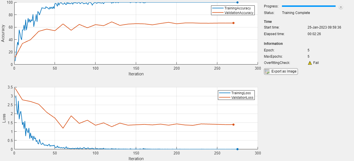
Check for Overfitting

Find the last value of the overfitting check for the model.

trainingCheck.LastValue

ans = 0

A LastValue value of 0 means that the model is overfitting. To prevent overfitting, try one or more of the following:

Randomize the data
Use data augmentation
Use dropout layers
Increase the regularization factor.

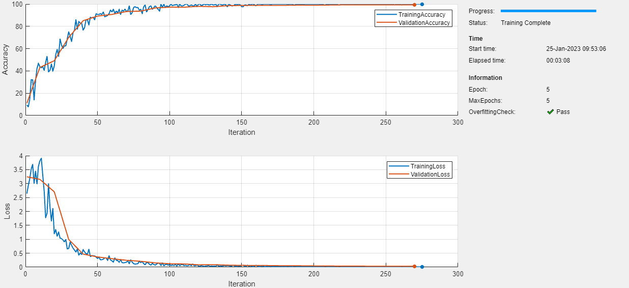
In this example, to prevent overfitting, randomize your data before training. To randomize the data, specify "randomized" when using the splitEachLabel function.

[imdsTrain,imdsValidation] = splitEachLabel(imds,trainingProportion,"randomized");

If you train the model again with the data randomized, then the model passes the overfitting check.

Supporting Functions

Model Loss Function

The modelLoss function takes a dlnetwork object net, a mini-batch of input data X with corresponding targets T and returns the loss, the gradients of the loss with respect to the learnable parameters in net, and the network state. To compute the gradients automatically, use the dlgradient function.

function [loss,gradients,state] = modelLoss(net,X,T)

% Forward data through network.
[Y,state] = forward(net,X);

% Calculate cross-entropy loss.
loss = crossentropy(Y,T);

% Calculate gradients of loss with respect to learnable parameters.
gradients = dlgradient(loss,net.Learnables);

end

Validation Metrics Function

The calculateValidationMetrics function takes a network, augmentedImageDatastore object containing the validation data, mini-batch size, and classes, and returns the loss and accuracy for the validation data.

function [loss,accuracy] = calculateValidationMetrics(net,augvalDatastore,miniBatchSize,classes)

% Pass the validation data through the network in batches.
mbq = minibatchqueue(augvalDatastore, ...
    MiniBatchSize=miniBatchSize, ...
    MiniBatchFcn=@preprocessMiniBatch, ...
    MiniBatchFormat=["SSCB",""]);

T = [];
Y = [];

% Loop over mini-batches.
while hasdata(mbq)
    [X,batchT] = next(mbq);

    % Pass the data through the network.
    batchY = predict(net,X);

    % Append to the output.
    Y = [Y,batchY];
    T = [T,batchT];
end

% Calculate the cross-entropy loss.
loss = crossentropy(Y,T);

% Compute the accuracy.
accuracy = 100*mean(onehotdecode(Y,classes,1) == onehotdecode(T,classes,1));

end

Mini-Batch Preprocessing Function

The preprocessMiniBatch function preprocesses a mini-batch of predictors and labels using the following steps:

Preprocess the images using the preprocessMiniBatchPredictors function.
Extract the label data from the incoming cell array and concatenate into a categorical array along the second dimension.
One-hot encode the categorical labels into numeric arrays. Encoding into the first dimension produces an encoded array that matches the shape of the network output.

function [X,T] = preprocessMiniBatch(dataX,dataT)

% Preprocess predictors.
X = preprocessMiniBatchPredictors(dataX);

% Extract label data from cell and concatenate.
T = cat(2,dataT{1:end});

% One-hot encode labels.
T = onehotencode(T,1);

end

Mini-Batch Predictors Preprocessing Function

The preprocessMiniBatchPredictors function preprocesses a mini-batch of predictors by extracting the image data from the input cell array and concatenating it into a numeric array. For grayscale input, concatenating over the fourth dimension adds a third dimension to each image, to use as a singleton channel dimension.

function X = preprocessMiniBatchPredictors(dataX)

% Concatenate.
X = cat(4,dataX{1:end});

end

Initialize Training Check

The showCheckOnPlot function creates a struct with information that you can use to update the overfitting check during training.

Name — Display name of the check in the training progress monitor window.
CheckFunction — Function handle to use to check for issues. For more information, see the checkForOverfitting function.

The function adds the check to the TrainingProgressMonitor object and displays the result in the Training Progress window. You can add more checks to the struct by defining more check functions and adding them to the struct.

function trainingCheck = showCheckOnPlot(monitor,threshold)

trainingCheck = struct("Name","OverfittingCheck", ...
    "CheckFunction",@(x)checkForOverfitting(x,threshold));

% Create an info item on the training progress monitor for the
% training check.
monitor.Info = [monitor.Info trainingCheck.Name];
updateInfo(monitor,trainingCheck.Name,"❓ Unknown");

end

Update Training Check

The updateTrainingChecks function takes as input a TrainingProgressMonitor object and a training check. The function verifies if the check passes by calling CheckFunction and updates LastValue with the result. If the check passes, then the check value is 1 and no issue was detected. If the check fails, then the check value is 0 and an issue was detected. The function updates the training progress monitor with the latest results.

function trainingCheck = updateTrainingChecks(monitor,trainingCheck)

% Update the training check.
check = trainingCheck.CheckFunction(monitor.MetricData);
if check == 0
    % Check failed.
    updateInfo(monitor,trainingCheck.Name,"⚠️ Fail");
    trainingCheck.LastValue = 0;
elseif check == 1
    % Check passed.
    updateInfo(monitor,trainingCheck.Name,"✔️ Pass")
    trainingCheck.LastValue = 1;
else
    % Check unverified. Use the existing value
    % in the Info field.
end

end

Overfitting Check Function

This checkForOverfitting function takes metric data containing the training and validation accuracy and determines if the model is not overfitting by checking if the ratio of validation accuracy to training accuracy is greater than or equal to the threshold given.

function result = checkForOverfitting(metricData,threshold)

% Set the number of training points to average the check across.
n = 10;

% If there is no value for one or other of the training or validation
% accuracies, then return unknown.
trainingAccData = metricData.TrainingAccuracy;
if size(trainingAccData,1) < n
    result = -1;
else
    % Check that the ratio of the last validation accuracy
    % to the average of the last 'n' training accuracy is
    % greater than the chosen threshold.
    avgTrainAcc = mean(trainingAccData(end-n+1:end));
    validationAccData = metricData.ValidationAccuracy;
    lastValidationAccPoint = validationAccData(end,:);
    result = lastValidationAccPoint(2)/avgTrainAcc >= threshold;
end

end