Explore Network Predictions Using Deep Learning Visualization Techniques
This example shows how to investigate network predictions using deep learning visualization techniques.
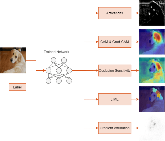
Deep learning networks are often described as "black boxes" because why a network makes a certain decision is not always obvious. You can use an interpretability technique to translate network behavior into output that a person can interpret. This interpretable output can then answer questions about the predictions of a network. This example focuses on visualization methods, which are interpretability techniques that explain network predictions using visual representations of what a network is “looking” at.
Load Pretrained Network
Load a pretrained GoogLeNet network and the corresponding class names. This requires the Deep Learning Toolbox™ Model for GoogLeNet Network support package. If this support package is not installed, then the software provides a download link. For a list of all available networks, see Pretrained Deep Neural Networks.
[net,classNames] = imagePretrainedNetwork("googlenet");Find the input size of the network.
inputSize = net.Layers(1).InputSize(1:2);
Classify Image
Load a test image containing a picture of a golden retriever.
img = imread("sherlock.jpg");
img = imresize(img,inputSize);

figure
imshow(img)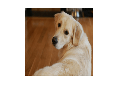
Classify the image using the pretrained network.
scores = minibatchpredict(net,img);
YPred = scores2label(scores,classNames)
YPred = categorical
     golden retriever
The network correctly classifies the image as a golden retriever. Find the three classes with the highest scores.
[~,topIdx] = maxk(scores,3);
topScores = scores(topIdx)';
topClasses = classNames(topIdx);
table(topClasses,topScores)
ans=3×2 table
         topClasses         topScores
    ____________________    _________

    "golden retriever"       0.55423
    "Labrador retriever"     0.39625
    "kuvasz"                0.025481
The classes with the top three scores are all dog breeds. The network outputs higher scores for the classes that share similar features with the true golden retriever class.
You can use visualization techniques to understand why the network classifies this image as a golden retriever.
Activation Visualization
One of the simplest ways of understanding network behavior is to visualize the activations of each layer. Most convolutional neural networks learn to detect features such as color and edges in their first convolutional layer. In deeper convolutional layers, the network learns to detect more complicated features, such as eyes. Pass the image through the network and examine the output activations of the conv2-relu_3x3_reduce layer.
act = minibatchpredict(net,img,Outputs="conv2-relu_3x3_reduce");
sz = size(act);
act = reshape(act,[sz(1) sz(2) 1 sz(3)]);
Display the activations for the first 12 channels of the layer.
I = imtile(mat2gray(act(:,:,:,1:12)));
figure
imshow(I)
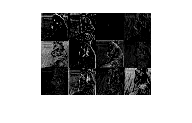
White pixels represent strong positive activations and black pixels represent strong negative activations. You can see that the network is learning low-level features, such as edges and texture. The first channel highlights the eyes and nose of the dog, possibly due to their distinctive edge and color.
Investigate a deeper layer.
actDeep = minibatchpredict(net,img,Outputs="inception_5b-output");
sz = size(actDeep)
sz = 1×3
7 7 1024
actDeep = reshape(actDeep,[sz(1) sz(2) 1 sz(3)]);
This layer has 1024 channels. Each channel has an image. Investigating every image in detail is impractical. Instead, you can gain insight into the network behavior by considering the channel with the strongest activation.
[maxValue,maxValueIndex] = max(max(max(actDeep)));
actDeepMax = actDeep(:,:,:,maxValueIndex);

tiledlayout("flow")
nexttile
imshow(img)
nexttile
imshow(imresize(mat2gray(actDeepMax),inputSize))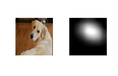
The strongest activating channel focuses on the head of the dog, indicating that this layer is picking out more complex features.
To further explore network behavior, you can use more complex visualization methods.
Grad-CAM
Explore the network predictions using gradient-weighted class activation mapping (Grad-CAM). To understand which parts of the image are most important for classification, Grad-CAM uses the gradient of the classification score with respect to the convolutional features determined by the network. The places where this gradient is large are exactly the places where the final score depends most on the data. Compute the Grad-CAM map using the gradCAM function and the predicted class.
channel = find(YPred == categorical(classNames));
gradcamMap = gradCAM(net,img,channel);
By default, the gradCAM function extracts the feature maps from the last ReLU layer with nonsingleton spatial dimensions or the last layer that gathers the outputs of ReLU layers (such as depth concatenation or addition layers). You can compute the Grad-CAM map for earlier layers in the network by specifying the feature layer. Compute the Grad-CAM map for the early convolutional layer conv2-relu_3x3.
gradcamMapShallow = gradCAM(net,img,channel,FeatureLayer="conv2-relu_3x3");Use the plotMaps supporting function, listed at the end of this example, to compare the Grad-CAM maps.
figure
alpha = 0.5;
cmap = "jet";
plotMaps(img,gradcamMap,gradcamMapShallow,"Deep Layer","Shallow Layer",alpha,cmap)
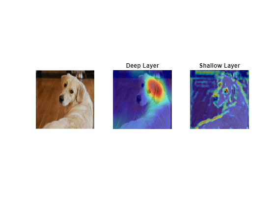
The Grad-CAM map for the layer at the end of the network highlights the head and ear of the dog, suggesting that the shape of the ear and the eye are important for classifying this dog as a golden retriever. The Grad-CAM map produced by the earlier layer highlights the edges of the dog. This is because earlier layers in a network learn simple features such as color and edges, while deep layers learn more complex features such as ears or eyes.
Occlusion Sensitivity
Compute the occlusion sensitivity of the image. Occlusion sensitivity is a simple technique for measuring network sensitivity to small perturbations in the input data. This method perturbs small areas of the input by replacing it with an occluding mask, typically a gray square. The mask moves across the image and the change in probability score for a given class is measured. You can use this method to highlight which parts of the image are most important to the classification. You can perform occlusion sensitivity using occlusionSensitivity.
Compute the occlusion sensitivity map for the golden retriever class.
occlusionMap = occlusionSensitivity(net,img,channel);
To examine the results of occlusion with higher resolution, reduce the mask size and stride using the MaskSize and Stride options. A smaller Stride value yields a higher resolution map but can take longer to compute and use more memory. A smaller MaskSize value yields more detail but can lead to noisier results. To get the best results from occlusion sensitivity, you must carefully choose the right values for the MaskSize and Stride options.
occlusionMapDetail = occlusionSensitivity(net,img,channel,Stride=10,MaskSize=15);
Use the plotMaps function to compare the different occlusion sensitivity results.
plotMaps(img,occlusionMap,occlusionMapDetail, ...
    "Occlusion Sensitivity","Occlusion Sensitivity \newline (High Resolution)",alpha,cmap)
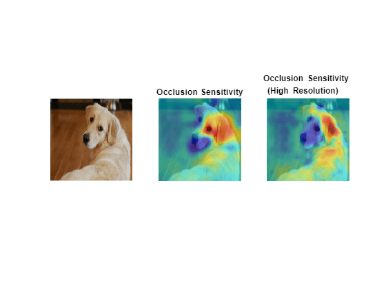
The lower resolution map shows similar results to Grad-CAM, highlighting the ear and eye of the dog. The higher resolution map shows that the ear is most important to the classification. The higher resolution map also indicates that the fur on the back of the dog is contributing to the classification decision.
LIME
Next, consider the locally interpretable model-agnostic explanations (LIME) technique. LIME approximates the classification behavior of a deep neural network using a simpler, more interpretable model, such as a regression tree. Interpreting the decisions of this simpler model provides insight into the decisions of the neural network. The simple model is used to determine the importance of features of the input data, as a proxy for the importance of the features to the deep neural network. The LIME technique uses a very different underlying mechanism to occlusion sensitivity or Grad-CAM.
Use the imageLIME function to view the most important features in the classification decision of a deep network. Compute the LIME map for the top two classes: golden retriever and Labrador retriever.
channel = find(ismember(classNames,topClasses));
limeMapClass1 = imageLIME(net,img,channel(1));
limeMapClass2 = imageLIME(net,img,channel(2));

titleClass1 = "LIME (" + string(channel(1)) + ")";
titleClass2 = "LIME (" + string(channel(2)) + ")";
plotMaps(img,limeMapClass1,limeMapClass2,titleClass1,titleClass2,alpha,cmap)
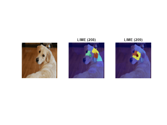
The maps show which areas of the image are important to the classification. Red areas of the map have a higher importance—an image lacking these areas would have a lower score for the specified class. For the golden retriever class, the network focuses on the dog's head and ear to make its prediction. For the Labrador retriever class, the network is more focused on the dog's nose and eyes, rather than the ear. While both maps highlight the dog's forehead, for the network, the dog's ear and neck indicate the golden retriever class, while the dog's eyes indicate the Labrador retriever class.
The LIME maps are consistent with the occlusion sensitivity and Grad-CAM maps. Comparing the results of different interpretability techniques is important for verifying the conclusions you make.
Gradient Attribution
Gradient attribution methods produce pixel-resolution maps showing which pixels are most important to the network classification decision. These methods compute the gradient of the class score with respect to the input pixels. Intuitively, the map shows which pixels most affect the class score when changed. The gradient attribution methods produce maps with a higher resolution than those from Grad-CAM or occlusion sensitivity, but that tends to be much noisier, as a well-trained deep network is not strongly dependent on the exact value of specific pixels.
Use the gradientAttribution supporting function, listed at the end of this example, to compute the gradient attribution map for the golden retriever class.
softmaxName = "prob";
pixelMap = gradientAttribution(net,img,YPred,softmaxName,"autodiff");
You can obtain a sharper gradient attribution map by modifying the backward pass through ReLU layers so that elements of the gradient that are less than zero and elements of the input to the ReLU layer that are less than zero are both set to zero. This method is known as guided backpropagation. Compute the gradient attribution map for the network using guided backpropagation.
pixelGuidedBackpropMap = gradientAttribution(net,img,YPred,softmaxName,"guided-backprop");Display the gradient attribution maps using a custom colormap with 255 colors that maps values of 0 to white and 1 to black. The darker pixels are those most important for classification.
alpha = 1;
cmap = [linspace(1,0,255)' linspace(1,0,255)' linspace(1,0,255)'];
plotMaps(img,pixelMap,pixelGuidedBackpropMap, ...
    "Gradient Attribution","Guided Backpropagation",alpha,cmap)
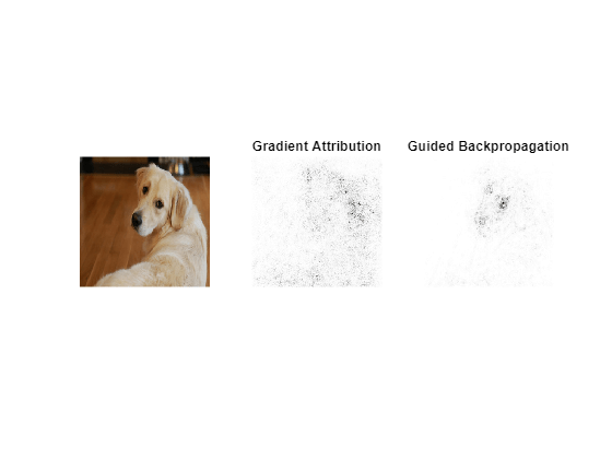
The darkest parts of the map are those centered around the dog. The map is very noisy, but it does suggest that the network is using the expected information in the image to perform classification. The pixels in the dog have much more impact on the classification score than the pixels of the background. In the guided backpropagation map, the pixels are focused on the face of the dog, specifically the eyes and nose. Interestingly, this method highlights different regions than the lower resolution visualization techniques. The result suggests that, at a pixel level, the nose and eyes of the dog are important for classifying the image as a golden retriever.
Deep Dream Image
Deep dream is a feature visualization technique that creates images that strongly activate network layers. By visualizing these images, you can highlight the image features learned by a network. These images are useful for understanding and diagnosing network behavior. You can generate images by visualizing the features of the layers toward the end of the network. Unlike the previous methods, this technique is global and shows you the overall behavior of the network, not just for a specific input image.
To produce images that resemble a given class most closely, use the final fully connected layer loss3-classifier. Generate deep dream images for the top three classes the network predicts for the test image. Set 'Verbose' to false to suppress detailed information on the optimization process.
channels = topIdx;
learnableLayer =  "loss3-classifier";
dreamImage = deepDreamImage(net,learnableLayer,channels,Verbose=false);
Increasing the number of pyramid levels and iterations per pyramid level can produce more detailed images at the expense of additional computation. Generate detailed deep dream images.
dreamImageDetailed = deepDreamImage(net,learnableLayer,channels, ...
    Verbose=false,NumIterations=100,PyramidLevels=4);
Compare the deep dream images of the top three classes.
tiledlayout(2,3)

for i = 1:3
nexttile
imshow(dreamImage(:,:,:,i));
title(string(topClasses(i)));
end

for i = 1:3
nexttile
imshow(dreamImageDetailed(:,:,:,i));
title(string(topClasses(i)) + "\newline (High Resolution)");
end
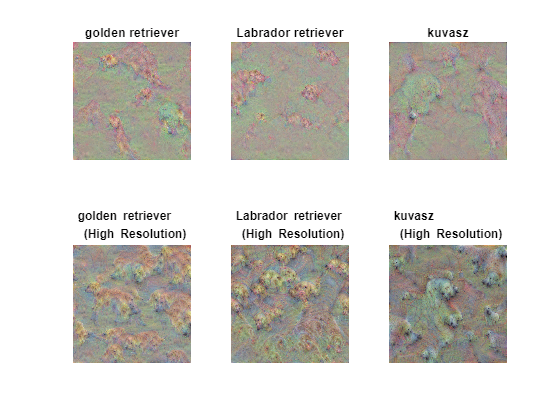
The deep dream images show how the network envisions each of the three classes. Although these images are quite abstract, you can see key features for each of the top classes. It also shows how the network distinguishes the golden and Labrador retriever classes.
To explore applying these methods interactively using an app, see the Explore Deep Network Explainability Using an App GitHub® repository.
Supporting Functions
Replace Layers Function
The replaceLayersOfType function replaces all layers of the specified class with instances of a new layer. The new layers have the same names as the original layers.
function net = replaceLayersOfType(net,layerType,newLayer)

% Replace layers in the dlnetwork net of the type specified by
% layerType with copies of the layer newLayer.

for i=1:length(net.Layers)
    if isa(net.Layers(i),layerType)
        % Match names between the old and new layers.
        layerName = net.Layers(i).Name;
        newLayer.Name = layerName;

        net = replaceLayer(net,layerName,newLayer);
    end
end
end
Plot Maps
Plot two maps, map1 and map2, for the input image img. Use alpha to set the transparency of the map. Specify which colormap to use using cmap.
function plotMaps(img,map1,map2,title1,title2,alpha,cmap)

figure
subplot(1,3,1)
imshow(img)

subplot(1,3,2)
imshow(img)
hold on
imagesc(map1,'AlphaData',alpha)
colormap(cmap)
title(title1)
hold off

subplot(1,3,3)
imshow(img)
hold on
imagesc(map2,'AlphaData',alpha)
colormap(cmap)
title(title2)
hold off
end
Gradient Attribution Map
Compute the gradient attribution map. You must specify the softmax layer. You can compute the basic map, or a higher resolution map using guided backpropagation.
function map = gradientAttribution(net,img,YPred,softmaxName,method)

% To use automatic differentiation, convert the image to a dlarray.
dlImg = dlarray(single(img),"SSC");

if method == "autodiff"
% Use dlfeval and the gradientMap function to compute the derivative. The gradientMap
% function passes the image forward through the network to obtain the class scores
% and contains a call to dlgradient to evaluate the gradients of the scores with respect
% to the image.
dydI = dlfeval(@gradientMap,net,dlImg,softmaxName,YPred);
end

if method == "guided-backprop"

% Use the custom layer CustomBackpropReluLayer (attached as a supporting file)
% with a nonstandard backward pass, and use it with automatic differentiation.
customRelu = CustomBackpropReluLayer();

% Set the BackpropMode property of each CustomBackpropReluLayer to "guided-backprop".
customRelu.BackpropMode = "guided-backprop";

% Use the supporting function replaceLayersOfType to replace all instances of reluLayer in the network with
% instances of CustomBackpropReluLayer.
net = replaceLayersOfType(net, ...
    'nnet.cnn.layer.ReLULayer',customRelu);

net = initialize(net);

dydI = dlfeval(@gradientMap,net,dlImg,softmaxName,YPred);
end

% Sum the absolute values of each pixel along the channel dimension, then rescale
% between 0 and 1.
map = sum(abs(extractdata(dydI)),3);
map = rescale(map);
end
Gradient Map
Compute the gradient of a class score with respect to one or more input images.
function dydI = gradientMap(net,dlImgs,softmaxName,classIdx)

dydI = dlarray(zeros(size(dlImgs)));

for i=1:size(dlImgs,4)
    I = dlImgs(:,:,:,i);
    scores = predict(net,I,Outputs=softmaxName);
    classScore = scores(classIdx);
    dydI(:,:,:,i) = dlgradient(classScore,I);
end
end
References
[1] Zhou, Bolei, Aditya Khosla, Agata Lapedriza, Aude Oliva, and Antonio Torralba. "Learning Deep Features for Discriminative Localization." In 2016 Proceedings of the IEEE Conference on Computer Vision and Pattern Recognition: 2921–29. Las Vegas, NV, USA: IEEE, 2016. https://doi.org/10.1109/CVPR.2016.319.
[2] Selvaraju, Ramprasaath R., Michael Cogswell, Abhishek Das, Ramakrishna Vedantam, Devi Parikh, and Dhruv Batra. “Grad-CAM: Visual Explanations from Deep Networks via Gradient-Based Localization.” In 2017 Proceedings of the IEEE Conference on Computer Vision: 618–626. Venice, Italy: IEEE, 2017. https://doi.org/10.1109/ICCV.2017.74.
[3] Ribeiro, Marco Tulio, Sameer Singh, and Carlos Guestrin. “‘Why Should I Trust You?’: Explaining the Predictions of Any Classifier.” In Proceedings of the 22nd ACM SIGKDD International Conference on Knowledge Discovery and Data Mining (2016): 1135–1144. New York, NY: Association for Computing Machinery, 2016. https://doi.org/10.1145/2939672.2939778.
[4] Simonyan, Karen, Andrea Vedaldi, and Andrew Zisserman. “Deep Inside Convolutional Networks: Visualising Image Classification Models and Saliency Maps.” Preprint, submitted April 19, 2014. https://arxiv.org/abs/1312.6034.
[5] TensorFlow. "DeepDreaming with TensorFlow." https://github.com/tensorflow/docs/blob/master/site/en/tutorials/generative/deepdream.ipynb.
See Also
gradCAM | imageLIME | occlusionSensitivity | deepDreamImage | tsne (Statistics and Machine Learning Toolbox)