Lowpass FIR Filter Design

A Lowpass FIR Filter Design Using Various Windows

FIR filters are widely used due to the powerful design algorithms that exist for them, their inherent stability when implemented in non-recursive form, the ease with which one can attain linear phase, their simple extensibility to multirate cases, and the ample hardware support that exists for them among other reasons. This example showcases functionality in the DSP System Toolbox™ for the design of low pass FIR filters with a variety of characteristics. Many of the concepts presented here can be extended to other responses such as highpass, bandpass, etc.

Consider a simple design of a lowpass filter with a cutoff frequency of 0.4*pi radians per sample:

Fc = 0.4;
N = 100;
Hf = fdesign.lowpass('N,Fc',N,Fc);

We can design this lowpass filter using the window method. For example, we can use a Hamming window or a Dolph-Chebyshev window:

Hd1 = design(Hf,'window','window',@hamming,SystemObject=true);
Hd2 = design(Hf,'window','window',{@chebwin,50}, ...
            SystemObject=true);
filterAnalyzer(Hd1,Hd2,FilterNames=["HammingWindowDesign","DolphChebyshevWindowDesign"]);

The choice of filter was arbitrary. Since ideally the order should be infinite, in general, a larger order results in a better approximation to ideal at the expense of a more costly implementation. For instance, with a Dolph-Chebyshev window, we can decrease the transition region by increasing the filter order:

Hf.FilterOrder = 200;
Hd3 = design(Hf,'window','window',{@chebwin,50},...
            SystemObject=true);
filterAnalyzer(Hd2,Hd3,FilterNames=["DolphChebyshevWindowDesignOrder100","DolphChebyshevWindowDesignOrder200"]);

Minimum Order Lowpass Filter Design

In order to determine a suitable filter order, it is necessary to specify the amount of passband ripple and stopband attenuation that will be tolerated. It is also necessary to specify the width of the transition region around the ideal cutoff frequency. The latter is done by setting the passband edge frequency and the stopband edge frequency. The difference between the two determines the transition width.

Fp = 0.38;
Fst = 0.42;
Ap = 0.06;
Ast = 60;
setspecs(Hf,'Fp,Fst,Ap,Ast',Fp,Fst,Ap,Ast);

We can still use the window method, along with a Kaiser window, to design the low pass filter.

Hd4 = design(Hf,'kaiserwin',SystemObject=true);
measure(Hd4);

ans =

Sampling Frequency : N/A (normalized frequency)
Passband Edge      : 0.38                      
3-dB Point         : 0.39539                   
6-dB Point         : 0.4                       
Stopband Edge      : 0.42                      
Passband Ripple    : 0.016058 dB               
Stopband Atten.    : 60.092 dB                 
Transition Width   : 0.04      

One thing to note is that the transition width as specified is centered around the cutoff frequency of 0.4 pi. This will become the point at which the gain of the lowpass filter is half the passband gain (or the point at which the filter reaches 6 dB of attenuation).

Optimal Minimum Order Designs

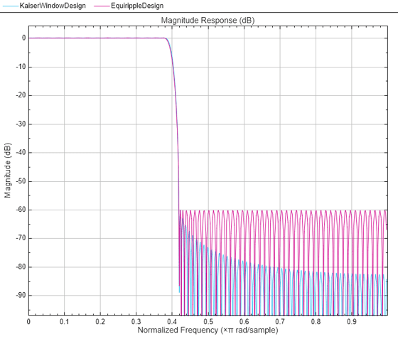
The Kaiser window design is not an optimal design and as a result the filter order required to meet the specifications using this method is larger than it needs to be. Equiripple designs result in the lowpass filter with the smallest possible order to meet a set of specifications.

Hd5 = design(Hf,'equiripple',SystemObject=true);
FA = filterAnalyzer(Hd4,Hd5,FilterNames=["KaiserWindowDesign","EquirippleDesign"]);

In this case, 146 coefficients are needed by the equiripple design while 183 are needed by the Kaiser window design.