Efficient Sample Rate Conversion Between Arbitrary Factors

Single Stage and Two-Stage Polyphase FIR Approach

Polyphase structures are generally considered efficient implementations of multirate filters. However in the case of fractional sample rate conversion, the number of phases, and therefore the filter order, can quickly become excessively high. For example, to resample a signal from 8 kHz to 44.1 kHz, we interpolate by 441 and decimate by 80 (8*441/80=44.1). A native single-stage FIR rate converter implementation requires 10560 coefficients.

FIRRC = designMultirateFIR(InterpolationFactor=441,DecimationFactor=80,...
                           StopbandAttenuation=50,SystemObject=true);
cost(FIRRC)

ans = struct with fields:
                  NumCoefficients: 10560
                        NumStates: 23
    MultiplicationsPerInputSample: 132
          AdditionsPerInputSample: 126.5000

This can be done much more efficiently in two stages, such as the design offered by the designRateConverter function.

SRC = designRateConverter(InputSampleRate=8e3,OutputSampleRate=44.1e3, ...
                            Bandwidth=6e3/2,StopbandAttenuation=50, Verbose=true);

designRateConverter(InputSampleRate=8000, OutputSampleRate=44100, Bandwidth=3000, StopbandAttenuation=50, MaxStages=Inf, CostMethod="estimate", Tolerance=0, ToleranceUnits="absolute")

Conversion ratio: 441:80
Input sample rate: 8000
Output sample rate: 44100

cost(SRC)

ans = struct with fields:
                  NumCoefficients: 1774
                        NumStates: 30
    MultiplicationsPerInputSample: 95.1750
          AdditionsPerInputSample: 89.6750

Although the number of operations per input sample is reasonable (roughly 95 multiplications - keeping in mind that the rate increases after the first stage to 14.7 kHz), 1774 coefficients would have to be stored in memory in this case.

Relaxing the Output Rate Tolerance

One way to mitigate the large number of coefficients could be to allow for a tolerance in the output sample rate if the exact rate is not critical. For example, specifying a tolerance of 1% results in an output rate of 44 kHz rather then 44.1 kHz. This now requires to interpolate by 11 and decimate by 2. It can be done efficiently with a single stage. In this case, 120 coefficients are needed and the number of multiplications per input sample is 60.

SRCWithTol = designRateConverter(InputSampleRate=8e3,OutputSampleRate=44.1e3, ...
                    StopbandAttenuation=50,Bandwidth=6e3/2, ...
                    Tolerance=1,ToleranceUnits='percentage',Verbose=true);

designRateConverter(InputSampleRate=8000, OutputSampleRate=44100, Bandwidth=3000, StopbandAttenuation=50, MaxStages=Inf, CostMethod="estimate", Tolerance=1, ToleranceUnits="percentage")

Conversion ratio: 11:2
Input sample rate: 8000
Output sample rate: 44100 (specified) 44000 (effective)

cost(SRCWithTol)

ans = struct with fields:
                  NumCoefficients: 120
                        NumStates: 12
    MultiplicationsPerInputSample: 60
          AdditionsPerInputSample: 55

Single Stage Farrow Approach

Polynomial-based filters are another way to overcome the problem of needing a large number of coefficients to be stored. Farrow structures are efficient implementations for such filters.

FRC3 = dsp.FarrowRateConverter(InputSampleRate=8e3, ...
    OutputSampleRate=44.1e3,PolynomialOrder=3);

FRC4 = dsp.FarrowRateConverter(InputSampleRate=8e3, ...
    OutputSampleRate=44.1e3,PolynomialOrder=4);

cost(FRC3)

ans = struct with fields:
                  NumCoefficients: 16
                        NumStates: 3
    MultiplicationsPerInputSample: 66.1500
          AdditionsPerInputSample: 60.6375

cost(FRC4)

ans = struct with fields:
                  NumCoefficients: 25
                        NumStates: 4
    MultiplicationsPerInputSample: 121.2750
          AdditionsPerInputSample: 99.2250

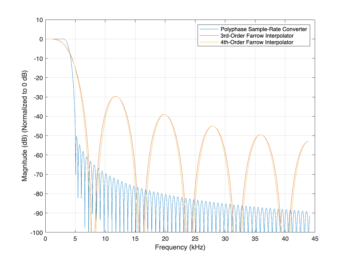
With 3rd-order polynomials, 16 coefficients are needed and about 66 multiplications per input sample. Fourth-order polynomials provide slightly better lowpass response at a higher cost: 25 coefficients and 121 multiplications per input sample. Plot the equivalent FIR frequency responses. The two-stage polyphase FIR design has a superior lowpass characteristics, with a sharper transition width.

F = linspace(0,44.1e3,2048);  % Define the frequency range analysis
Fs1 = 8e3*147;  % The equivalent single stage filter is clocked at 3.53 MHz

SRCmag  = freqz(SRC.Stage1,F,"half",Fs1);
FRC3mag = freqz(FRC3,F,"half",3*Fs1);
FRC4mag = freqz(FRC4,F,"half",3*Fs1);

plot(F/1e3,db(SRCmag/147));
hold on
plot(F/1e3,db(FRC3mag/441));
plot(F/1e3,db(FRC4mag/441));
hold off
xlabel("Frequency (kHz)")
ylabel("Magnitude (dB) (Normalized to 0 dB)")
legend(["Polyphase Sample-Rate Converter", ...
        "3rd-Order Farrow Interpolator","4th-Order Farrow Interpolator"]);
ylim([-100 10])
grid on

Use the freqzmr function to plot the DTFT of the impulse response of each filter. These plots suggest how the spectra of typical output signals look like. The ideal output spectrum is a flat lowpass signal between 0 and 4kHz, but the limitations of FIR and Farrow filtering cause some transition effects and a nonzero stopband. Nevertheless, the sample rate converter has a superior transition and stopband performance in the output spectrum.

[SRCoutMag,SRCFreq]   = freqzmr(SRC);
[FRC3outMag,FRC3Freq] = freqzmr(FRC3);
[FRC4outMag,FRC4Freq] = freqzmr(FRC4);

plot(SRCFreq/1e3,db(SRCoutMag)); 
hold on
plot(FRC3Freq/1e3,db(FRC3outMag)); 
plot(FRC4Freq/1e3,db(FRC4outMag)); 
hold off

legend(["Polyphase Sample-Rate Converter", ...
        "3rd-Order Farrow Interpolator",...
        "4th-Order Farrow Interpolator"])
xlabel("Frequency (kHz)")
ylabel("Magnitude (dB)")

Providing an output rate tolerance does not significantly impact the implementation cost of the Farrow filter. However, it does change the interpolation and decimation factors in the same way it does for the previous multi-stage FIR design.

FRC_4thWithTol = dsp.FarrowRateConverter(InputSampleRate=8e3, ...
    OutputSampleRate=44.1e3,PolynomialOrder=4, ...
    OutputRateTolerance=0.01);
info(FRC_4thWithTol)

ans = 12×52 char array
    'Discrete-Time FIR Multirate Filter (real)           '
    '-----------------------------------------           '
    'Filter Structure      : Farrow Sample-Rate Converter'
    'Interpolation Factor  : 11                          '
    'Decimation Factor     : 2                           '
    'Filter Length         : 5                           '
    'Stable                : Yes                         '
    'Linear Phase          : No                          '
    '                                                    '
    'Arithmetic            : double                      '
    'Output Rate Tolerance : 1.000000 %                  '
    'Adjusted Output Rate  : 44000.000000                '

cost(FRC_4thWithTol)

ans = struct with fields:
                  NumCoefficients: 25
                        NumStates: 4
    MultiplicationsPerInputSample: 121
          AdditionsPerInputSample: 99

Cascade of Farrow and FIR Polyphase Structures

We now try to design a hybrid solution that would take advantage of the two types of filters that we have previously seen. Polyphase filters are particularly well adapted for interpolation or decimation by an integer factor and for fractional rate conversions when the interpolation and the decimation factors are low. Farrow filters can efficiently implement arbitrary (including irrational) rate change factors. First, we interpolate the original 8 kHz signal by 4 using a cascade of FIR halfband filters.

intSRC = designRateConverter(InputSampleRate=8e3,OutputSampleRate=32e3, ...
    StopbandAttenuation=50,Bandwidth=6e3/2, Verbose=true);

designRateConverter(InputSampleRate=8000, OutputSampleRate=32000, Bandwidth=3000, StopbandAttenuation=50, MaxStages=Inf, CostMethod="estimate", Tolerance=0, ToleranceUnits="absolute")

Conversion ratio: 4:1
Input sample rate: 8000
Output sample rate: 32000

Then, we interpolate the intermediate 32 kHz signal by 44.1/32 = 1.378125 to get the desired 44.1 kHz final sampling frequency. We use a cubic Lagrange polynomial-based filter for this purpose.

FRC = dsp.FarrowRateConverter(InputSampleRate=32e3, ...
    OutputSampleRate=44.1e3,PolynomialOrder=3);

The overall filter is simply obtained by cascading the two filters.

cost(intSRC)

ans = struct with fields:
                  NumCoefficients: 34
                        NumStates: 11
    MultiplicationsPerInputSample: 34
          AdditionsPerInputSample: 31

cost(FRC)

ans = struct with fields:
                  NumCoefficients: 16
                        NumStates: 3
    MultiplicationsPerInputSample: 16.5375
          AdditionsPerInputSample: 15.1594

The number of nonzero and non-unity coefficients of this hybrid design is relatively low (34+12=46) and the number of multiplications per input sample is also relatively low (34 + 16.5375*4 ≈ 92).

hybrid = cascade(intSRC, FRC);
cost(hybrid)

ans = struct with fields:
                  NumCoefficients: 46
                        NumStates: 14
    MultiplicationsPerInputSample: 100.1500
          AdditionsPerInputSample: 91.6375

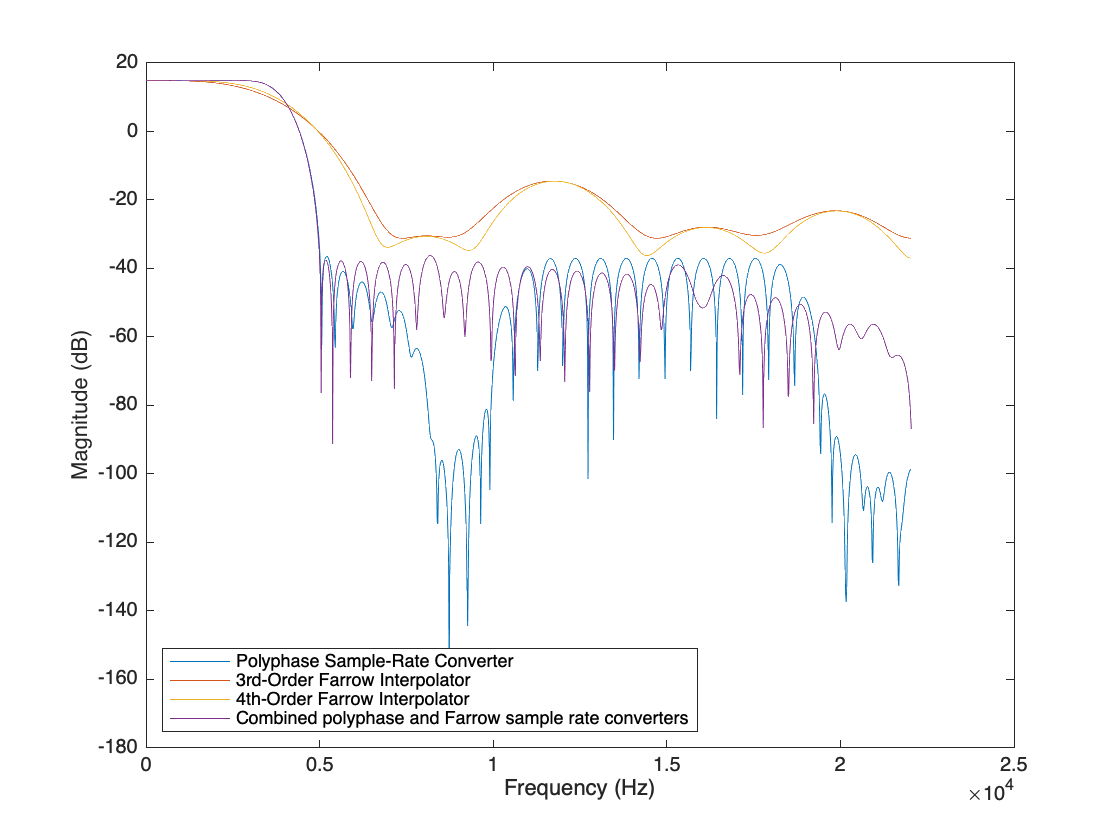
Overlay the frequency responses of the single-stage and the multistage designs. Clearly the multistage responses (hybrid and SRC) are comparable to each other, and are superior to the responses of the FRC3 and FRC4 filters.

[HybridOutMag, HybridFreq] = freqzmr(hybrid);
plot(SRCFreq,db(SRCoutMag)); 
hold on
plot(FRC3Freq,db(FRC3outMag));
plot(FRC4Freq,db(FRC4outMag)); 
plot(HybridFreq,db(HybridOutMag));
hold off

xlabel("Frequency (Hz)")
ylabel("Magnitude (dB)")
legend(["Polyphase Sample-Rate Converter", ...
        "3rd-Order Farrow Interpolator",...
        "4th-Order Farrow Interpolator",...
        "Combined polyphase and Farrow sample rate converters"],...
       Location="SouthWest")

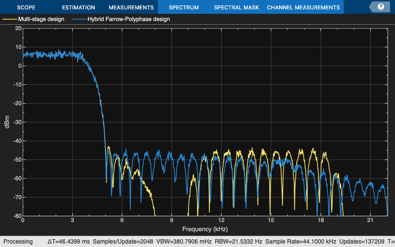
You can be verify the performance by empirical analysis of the response to a random white input excitation.

scope = spectrumAnalyzer(SampleRate=44.1e3,PlotAsTwoSidedSpectrum=false, ...
    YLimits=[-80 20],ShowLegend=true, ...
    ChannelNames=["Multi-stage design","Hybrid Farrow-Polyphase design"]);
tic,
while toc < 10
    % Run for 20 seconds
    x = randn(8000,1);
    
    % Convert rate using multistage FIR filters
    y1 = SRC(x);

    % Convert rate using cascade of multistage FIR and Farrow filter    
    y2 = hybrid(x);
   
    % Compare the output from both approaches
    scope([y1,y2])
end