Multistage Rate Conversion Using FIR Rate Converter
This example shows how to leverage multiple FIR Rate converters for sample rate conversion from 48 kHz to 44.1 kHz. In the multistage approach, we split the interpolation and decimation factors into simpler factors that reduce the combined filter order, reducing the computational complexity of the filtering process. The conversion of 48 kHz to 44.1 kHz can be performed in a single stage using interpolation factor L = 147 and decimation factor M = 160 or in multiple stages as described below:
Stage 1, L = 7 and M = 5 (48 kHz to 67.2 kHz)
Stage 2, L= 7 and M = 8 (67.2 kHz to 58.8 kHz)
Stage 3, L = 3 and M = 4 (58.8 kHz to 44.1 kHz)
Single-Stage v.s. Multistage Cost Analysis
We can cascade the three rate conversion stages to form a single-stage equivalent filter, which functions in the same manner as a single-stage FIR Rate converter. However, the multistage approach is more efficient in terms of memory because the cascaded rate converters use less memory (states and coefficients) than the single rate converter.
rcSingleStage = dsp.FIRRateConverter(InterpolationFactor=147,...
    DecimationFactor=160);
costSingleStage = cost(rcSingleStage)
costSingleStage = struct with fields:
NumCoefficients: 3507
NumStates: 24
MultiplicationsPerInputSample: 21.9187
AdditionsPerInputSample: 21
rcStage1 = dsp.FIRRateConverter(InterpolationFactor=7,...
    DecimationFactor=5);
rcStage2 = dsp.FIRRateConverter(InterpolationFactor=7,...
    DecimationFactor=8);
rcStage3 = dsp.FIRRateConverter(InterpolationFactor=3,...
    DecimationFactor=4);
rcMultiStage = dsp.FilterCascade(rcStage1,rcStage2,rcStage3);
costMultiStage = cost(rcMultiStage)
costMultiStage = struct with fields:
                  NumCoefficients: 348
                        NumStates: 70
    MultiplicationsPerInputSample: 71.7188
          AdditionsPerInputSample: 68.3750
Comparing the Frequency Response of Single-Stage and Multistage Approach
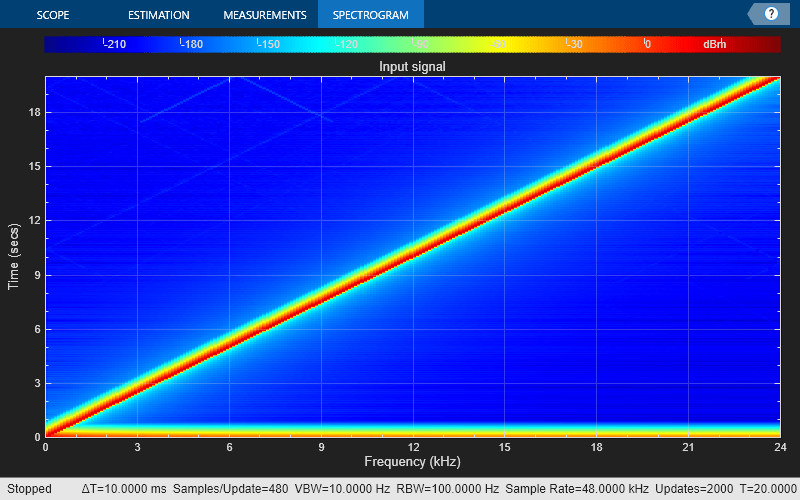
We use a chirp signal to compare the numerical accuracy between a single-stage rate converter and a cascaded multistage rate converter. To generate a chirp signal, we use a dsp.Chirp System object™. Initially, the frequency is set to 10 Hz which increases exponentially to 24 kHz at time t = 5 sec. The input signal is sampled at 48 kHz and each call to the dsp.Chirp System object returns an output of size 1600-by-1.
% Input sample rate
fsIn = 48e3;

% Output sample rate
fsOut = 441e2;

% Input Rows
inputFrameRows = 1000;

% Signal duration
Ts = 20;

% Creating a chirp signal sampled at 48 kHz
input = dsp.Chirp(Type="Linear",InitialFrequency=10,TargetFrequency=fsIn/2,...
    TargetTime=Ts,SweepTime=Ts,SamplesPerFrame=inputFrameRows,SampleRate=fsIn);
We can compare the frequency response between the single-stage and multistage rate conversion by using spectrumAnalyzer on the filtered outputs.
% Spectrum Analyzer to view the spectrogram of the input
scope1 = spectrumAnalyzer(ViewType="spectrogram",SampleRate=fsIn, ...
    PlotAsTwoSidedSpectrum=false, ...
    RBWSource="Property",RBW=100, ...
    VBWSource="Property",VBW=10, ...
    TimeSpanSource="Property",TimeSpan=Ts, ...
    Title="Input signal");

% Spectrum Analyzer to view the spectrogram of the single-stage filtered output
scope2 = spectrumAnalyzer(ViewType="spectrogram",SampleRate=fsOut, ...
    PlotAsTwoSidedSpectrum=false, ...
    RBWSource="Property",RBW=100, ...
    VBWSource="Property",VBW=10, ...
    TimeSpanSource="Property",TimeSpan=Ts, ...
    Title="Single-stage filtered output");

% Spectrum Analyzer to view the spectrogram of the multi-stage filtered output
scope3 = spectrumAnalyzer(ViewType="spectrogram",SampleRate=fsOut, ...
    PlotAsTwoSidedSpectrum=false, ...
    RBWSource="Property",RBW=100, ...
    VBWSource="Property",VBW=10, ...
    TimeSpanSource="Property",TimeSpan=Ts, ...
    Title="Multi-stage filtered output");

% Number of steps required to process a signal of duration 5 seconds
numSteps = Ts * fsIn / inputFrameRows;

% Filter the input of duration 5 seconds.
for i=1:numSteps

    x = input();

    ySingleStage = rcSingleStage(x);

    yMultiStage = rcMultiStage(x);

    scope1(x);

    scope2(ySingleStage);

    scope3(yMultiStage);

end
% Input signal
release(scope1)

% Single-stage rate converter output
release(scope2)
% Multistage rate converter output
release(scope3)
Incorrect Ordering of Rate Converters
To demonstrate the effect of incorrect ordering of rate converters in the multistage process, we reorder the stages leading to the following sample rate change:
Stage 1, L = 3 and M = 4 (48 kHz to 36 kHz)
Stage 2, L = 7 and M = 5 (36 kHz to 50.4 kHz)
Stage 3, L = 7 and M = 8 (50.4 kHz to 44.1 kHz)
This ordering of the filters leads to a cutoff frequency of 18 kHz in stage 1. The input signal contains valid frequencies up to 44.1/2 or 22.05 kHz. To avoid aliasing which results in signal content loss, the first FIR rate converter filters out the frequencies in the range 18 kHz to 22.05 kHz.
We use the same input as before to compare the response of the multistage rate conversion process against the reference single-stage rate conversion process. The output spectrogram of the incorrectly ordered filter shows signal content loss due to a drop in the sampling frequency below 44.1 kHz.
input.reset();

rcStage1.reset();
rcStage2.reset();
rcStage3.reset();

% Incorrect order
rcMultiStageIncorrect = dsp.FilterCascade(rcStage3,rcStage1,rcStage2);

% Use single-stage rate converter output as reference
rcSingleStage.reset()

% Spectrum Analyzer to view the spectrogram of the input
scope4 = spectrumAnalyzer(ViewType="spectrogram",SampleRate=fsIn, ...
    PlotAsTwoSidedSpectrum=false, ...
    RBWSource="Property",RBW=100, ...
    VBWSource="Property",VBW=10, ...
    TimeSpanSource="Property",TimeSpan=Ts, ...
    Title="Input signal");

% Spectrum Analyzer to view the spectrogram of the multi-stage filtered output
scope5 = spectrumAnalyzer(ViewType="spectrogram",SampleRate=fsOut, ...
    PlotAsTwoSidedSpectrum=false, ...
    RBWSource="Property",RBW=100, ...
    VBWSource="Property",VBW=10, ...
    TimeSpanSource="Property",TimeSpan=Ts, ...
    Title="Multi-stage filtered output");

% Spectrum Analyzer to view the spectrogram of the reference output
scope6 = spectrumAnalyzer(ViewType="spectrogram",SampleRate=fsOut, ...
    PlotAsTwoSidedSpectrum=false, ...
    RBWSource="Property",RBW=100, ...
    VBWSource="Property",VBW=10, ...
    TimeSpanSource="Property",TimeSpan=Ts, ...
    Title="Reference single-stage output signal");

% Filter the input of duration 5 seconds.
for i=1:numSteps

    x = input();

    yMultiStageIncorrect = rcMultiStageIncorrect(x);
    yRef = rcSingleStage(x);

    scope4(x);
    scope5(yMultiStageIncorrect);
    scope6(yRef);

end
% Input signal
release(scope4)
% Incorrect ordering of stages
release(scope5)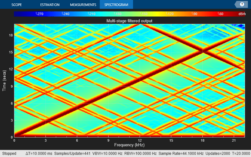
% Reference output
release(scope6)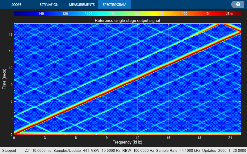
Conclusion
After comparing the two approaches, we can conclude that the multistage approach efficiently converts the input sample rate using a significantly smaller combined filter order. Note that the rate change factors, order of rate converters and filter specifications are chosen in a manner to minimize signal content loss through aliasing and imaging.