Cancel Noise Using Fully Serial LMS Filter
R2026bThis example shows how to cancel additive noise from a corrupted signal using the LMS Filter block in DSP HDL Toolbox™. You have a pure sine wave information signal corrupted by colored noise, and you use the serial direct form least mean square (LMS) architecture to adaptively filter a correlated noise reference, recovering the clean signal from the error output. The model in this example implements an adaptive noise cancellation system where the LMS Filter block receives a noisy desired signal and a correlated noise reference, then produces the noise-canceled information signal at its error output. In this example, you explore the fully serial direct form LMS architecture and its resource-efficient design for FPGA implementations.
Serial Direct Form Architecture
To implement an LMS adaptive filter on an FPGA with minimal hardware resources, choose serial direct form architecture. This trades throughput for area, making it suitable for applications where the input sample rate is much lower than the FPGA clock rate. The LMS Filter block in this model uses the Serial direct form LMS architecture. This block requires 2*  +
+  clock cycles to produce each output, where is the filter length and is additional pipeline latency.
Configure Filter Parameters
To achieve effective noise cancellation, you must choose the filter length and step size carefully. Configure filter length and step size to balance convergence speed against stability, and simulate the noise cancellation model and verify that the LMS filter recovers the information signal as it converges. The filter length determines how many taps the adaptive filter uses to model the noise path, and the step size controls how quickly the filter coefficients converge.
filterLength = 16;
stepSize = 0.01;
The filter length of 16 matches the order of the FIR filter that colors the noise in this scenario. If you know the length of the unknown system you are modeling, set the adaptive filter length to match it. Choose step size that satisfies the stability condition  < 1\(
< 1\( x ), where is the input signal power and is the filter length. A smaller step size provides more stable convergence at the cost of slower adaptation.
Prepare Input Signals
To test the noise cancellation system, create a scenario with a known information signal, a noise source, and a coloring filter that creates correlation between the noise reference and the noise component in the desired signal.
numOfSamples = 1000;
signal = sin(2*pi*0.04*(0:numOfSamples-1)');

filterObj = dsp.FIRFilter(Numerator=fir1(filterLength-1,0.5));
noise = 0.8*randn(numOfSamples,1);
desiredSignal = signal + filterObj(noise);
observedSignal = noise;
The desired signal combines the pure sine wave with colored noise. The observed signal (noise reference) feeds directly into the LMS filter input. As the adaptive filter converges, its output approximates the colored noise component in the desired signal. The error output, the difference between the desired signal and the filter output, yields the recovered information signal.
Simulate Model
To observe the noise cancellation behavior, compute the simulation time based on the filter latency and run the model. The serial architecture introduces latency proportional to the filter length, so the simulation must run long enough for all input samples to propagate through the system.
adaptIn = true(numOfSamples,1);
resetIn = false(numOfSamples,1);
validIn = true(numOfSamples,1);

lmsObj = dsphdl.LMSFilter(Architecture="Serial direct form LMS",FilterLength=filterLength);
lmsLatency = getLatency(lmsObj);
simtime = length(observedSignal)*(lmsLatency+1) + lmsLatency;

out = sim("HDLFullySerialLMS");
The getLatency method returns the number of clock cycles between a valid input and its corresponding valid output. You use this value to compute the total simulation time, ensuring every input sample produces a corresponding output.
Analyze Noise Cancellation Results
To verify that the LMS filter successfully recovers the information signal, compare the original sine wave, the noisy desired signal, and the error output. As the filter converges, the error signal progressively resembles the clean sine wave.
actErrorOut = squeeze(out.errorOut);
actErrorOut = actErrorOut(1:numOfSamples);

figure;
subplot(3,1,1)
plot(1:numOfSamples,signal(1:numOfSamples));
title("Cancel Noise Using Fully Serial LMS Filter")
subtitle("Information Signal")
xlabel("Sample Index")
ylabel("Signal Value")

subplot(3,1,2)
plot(1:numOfSamples,double(desiredSignal))
subtitle("Noisy Signal")
xlabel("Sample Index")
ylabel("Signal Value")

subplot(3,1,3)
plot(1:length(actErrorOut),double(actErrorOut));
subtitle("Noise Canceled Signal")
xlabel("Sample Index")
ylabel("Signal Value")
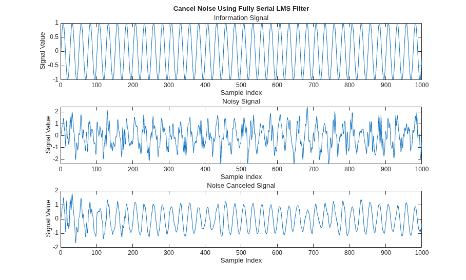
The top subplot shows the original pure sine wave. The middle subplot shows the desired signal corrupted by colored noise, which serves as the reference for the LMS algorithm. The bottom subplot shows the error output from the LMS filter. During the first 100-200 samples, the error signal still contains significant noise because the filter coefficients have not yet converged. After convergence, the error signal closely matches the original sine wave, confirming that the adaptive filter has learned the noise transfer path and effectively subtracted the noise component. A smaller step size produces a cleaner steady-state result but requires more samples to converge.

