Assess Collinearity Among Multiple Series Using Econometric Modeler App
This example shows how to assess the strengths and sources of
collinearity among multiple series by using Belsley collinearity diagnostics in the
Econometric Modeler app. The data set, stored in Data_Canada.mat,
contains annual Canadian inflation and interest rates from 1954 through 1994.
At the command line, load the Data_Canada.mat data
set.
load Data_CanadaAt the command line, open the Econometric Modeler app.
econometricModeler
Alternatively, open the app from the apps gallery (see Econometric Modeler).
Import DataTimeTable into the app:
On the Modeler tab, in the Import section, click the Import button
 .
.In the Import Data dialog box, select the check box for the
DataTimeTablevariable.Click Import.
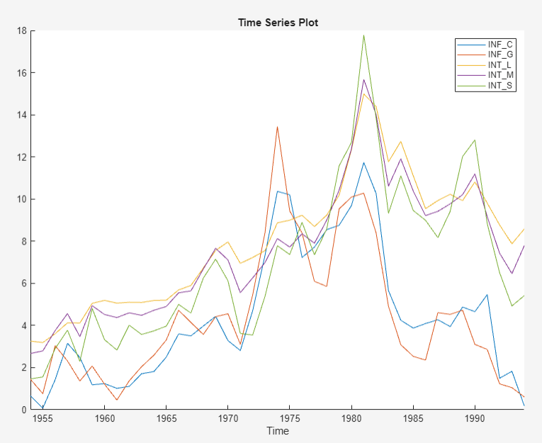
The Canadian interest and inflation rate variables appear in the Time Series pane, and a time series plot of all the series appears in the Plot(INF_C) figure window.
Perform Belsley collinearity diagnostics on all series. On the Modeler tab, in the Tests section, click Add Test > Belsley Collinearity Diagnostics.
The Collinearity(INF_C) document appear with the following results:
A table of singular values, corresponding condition indices, and corresponding variable variance-decomposition proportions
A plot of the variable variance-decomposition proportions corresponding to the condition index that is above the threshold, and a horizontal line indicating the variance-decomposition threshold
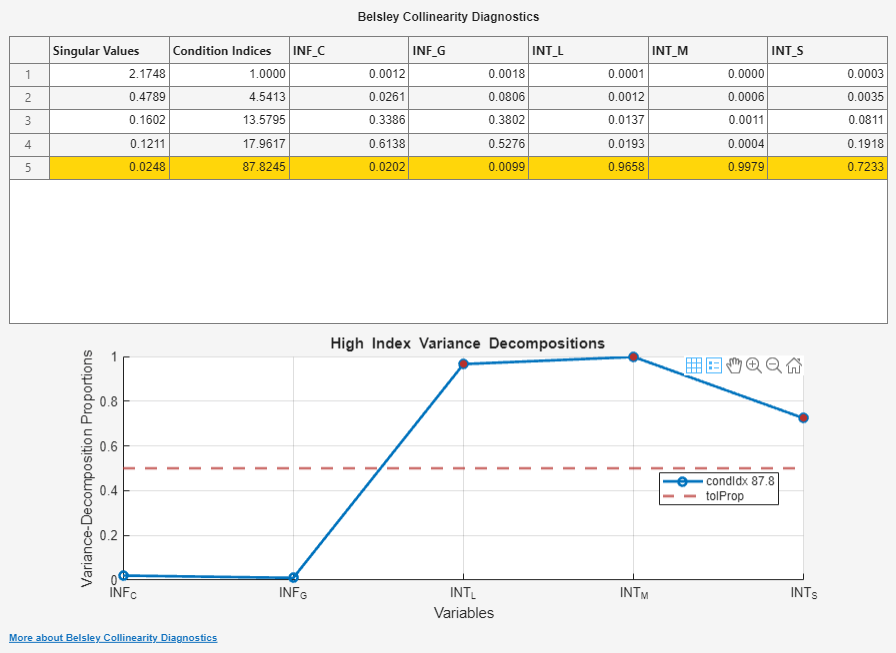
The interest rates have variance-decomposition proportions exceeding the default tolerance, 0.5, indicated by red markers in the plot. This result suggests that the interest rates exhibit multicollinearity. If you use the three interest rates as predictors in a linear regression model, then the predictor data matrix can be ill conditioned.