infer

Infer conditional variances of conditional variance models

Syntax

V = infer(Mdl,Y)

Tbl2 = infer(Mdl,Tbl1)

___
 = infer(___,Name,Value)

[___,logL] = infer(___)

Description

V = infer(Mdl,Y) returns a numeric array V containing the series of conditional variances from evaluating the fully specified, univariate conditional variance model Mdl at the numeric array of response data Y. Mdl can be a garch, egarch, or gjr model.

example

Tbl2 = infer(Mdl,Tbl1) returns the table or timetable Tbl2 containing the inferred conditional variances and innovations from evaluating the fully specified, univariate conditional variance model Mdl at the response variable data in the table or timetable Tbl1. When Mdl is a model fitted to the response data and returned by estimate, the inferred innovations are residuals. (since R2023a)

infer selects the response variable named in Mdl.SeriesName or the sole variable in Tbl1. To select a different response variable in Tbl1 at which to evaluate the model, use the ResponseVariable name-value argument.

example

___ = infer(___,Name,Value) specifies options using one or more name-value arguments in addition to any of the input argument combinations in previous syntaxes. infer returns the output argument combination for the corresponding input arguments. For example, infer(Mdl,Y,V0=v0) initializes the conditional variance model of Mdl using the presample conditional variance data in v0.

example

[___,logL] = infer(___) also returns the loglikelihood objective function values logL associated with each inferred path.

example

Examples

collapse all

Infer GARCH Model Conditional Variances From Numeric Response Data

Open Script

Infer conditional variances from a GARCH(1,1) model with known coefficients. Specify response data as a numeric vector.

Specify a GARCH(1,1) model with known parameters. Simulate 101 conditional variances and responses (innovations) from the model. Set aside the first observation from each series to use as presample data.

Mdl = garch(Constant=0.01,GARCH=0.8,ARCH=0.15);

rng("default") % For reproducibility
[vS,yS] = simulate(Mdl,101);
y0 = yS(1);
v0 = vS(1);
y = yS(2:end);
v = vS(2:end);

figure
tiledlayout(2,1)
nexttile
plot(v)
title("Conditional Variances")
nexttile
plot(y)
title("Innovations")

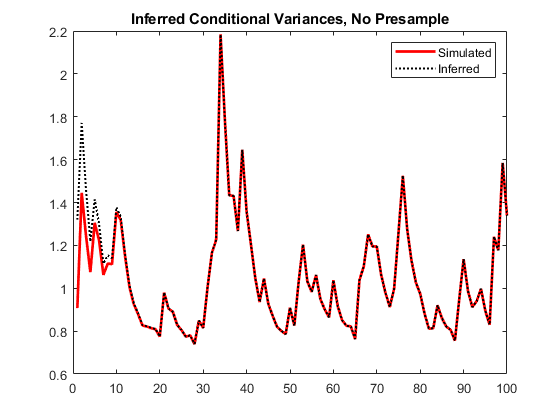
Infer the conditional variances of y without using presample data. Compare them to the known (simulated) conditional variances.

vI = infer(Mdl,y);

figure
plot(1:100,v,"r",LineWidth=2)
hold on
plot(1:100,vI,"k:",LineWidth=1.5)
legend("Simulated","Inferred",Location="northeast")
title("Inferred Conditional Variances, No Presample")
hold off

Notice the transient response (discrepancy) in the early time periods due to the absence of presample data.

Infer conditional variances using the set-aside presample innovation, y0. Compare them to the known (simulated) conditional variances.

vE = infer(Mdl,y,E0=y0);

figure
plot(1:100,v,"r",LineWidth=2)
hold on
plot(1:100,vE,"k:",LineWidth=1.5)
legend("Simulated","Inferred",Location="northeast")
title("Inferred Conditional Variances, Innovations Presample")
hold off

There is a slightly reduced transient response in the early time periods.

Infer conditional variances using the presample of conditional variance data, v0. Compare them to the known (simulated) conditional variances.

vO = infer(Mdl,y,V0=v0);

figure
plot(v)
plot(1:100,v,"r",LineWidth=2)
hold on
plot(1:100,vO,"k:",LineWidth=1.5)
legend("Simulated","Inferred",Location="northeast")
title("Inferred Conditional Variances, Conditional Variance Presample")
hold off

There is a much smaller transient response in the early time periods.

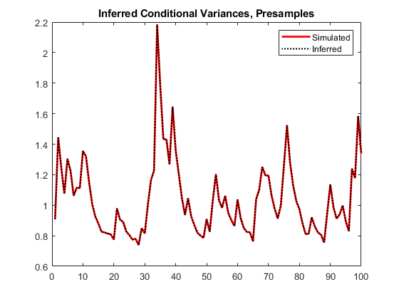
Infer conditional variances using both the presample innovation and conditional variance. Compare them to the known (simulated) conditional variances.

vEO = infer(Mdl,y,E0=y0,V0=v0);

figure
plot(v)
plot(1:100,v,"r",LineWidth=2)
hold on
plot(1:100,vEO,"k:",LineWidth=1.5)
legend("Simulated","Inferred",Location="northeast")
title("Inferred Conditional Variances, Presamples")
hold off

When you use sufficient presample innovations and conditional variances, the inferred conditional variances are exact (there is no transient response).

Infer EGARCH Model Conditional Variances

Open Script

Infer conditional variances from an EGARCH(1,1) model with known coefficients. When you use, and then do not use presample data, compare the results from infer.

Specify an EGARCH(1,1) model with known parameters. Simulate 101 conditional variances and responses (innovations) from the model. Set aside the first observation from each series to use as presample data.

Mdl = egarch(Constant=0.001,GARCH=0.8, ...
    ARCH=0.15,Leverage=-0.1);

rng("default") % For reproducibility
[vS,yS] = simulate(Mdl,101);
y0 = yS(1);
v0 = vS(1);
y = yS(2:end);
v = vS(2:end);

figure
tiledlayout(2,1)
nexttile
plot(v)
title("Conditional Variances")
nexttile
plot(y)
title("Innovations")

Infer the conditional variances of y without using any presample data. Compare them to the known (simulated) conditional variances.

vI = infer(Mdl,y);

figure
plot(1:100,v,"r",LineWidth=2)
hold on
plot(1:100,vI,"k:",LineWidth=1.5)
legend("Simulated","Inferred",Location="northeast")
title("Inferred Conditional Variances, No Presample")
hold off

Notice the transient response (discrepancy) in the early time periods due to the absence of presample data.

Infer conditional variances using the set-aside presample innovation, y0. Compare them to the known (simulated) conditional variances.

vE = infer(Mdl,y,E0=y0);

figure
plot(1:100,v,"r",LineWidth=2)
hold on
plot(1:100,vE,"k:",LineWidth=1.5)
legend("Simulated","Inferred",Location="northeast")
title("Inferred Conditional Variances, Presample E")
hold off

There is a slightly reduced transient response in the early time periods.

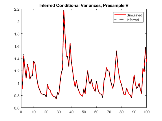
Infer conditional variances using the set-aside presample variance, v0. Compare them to the known (simulated) conditional variances.

vO = infer(Mdl,y,V0=v0);

figure
plot(v)
plot(1:100,v,"r",LineWidth=2)
hold on
plot(1:100,vO,"k:",LineWidth=1.5)
legend("Simulated","Inferred",Location="northeast")
title("Inferred Conditional Variances, Presample V")
hold off

The transient response is almost eliminated.

Infer conditional variances using both the presample innovation and conditional variance. Compare them to the known (simulated) conditional variances.

vEO = infer(Mdl,y,E0=y0,V0=v0);

figure
plot(v)
plot(1:100,v,"r",LineWidth=2)
hold on
plot(1:100,vEO,"k:",LineWidth=1.5)
legend("Simulated","Inferred",Location="northeast")
title("Inferred Conditional Variances, Presamples")
hold off

When you use sufficient presample innovations and conditional variances, the inferred conditional variances are exact (there is no transient response).

Infer GJR Model Conditional Variances

Open Script

Infer conditional variances from a GJR(1,1) model with known coefficients. When you use, and then do not use presample data, compare the results from infer.

Specify a GJR(1,1) model with known parameters. Simulate 101 conditional variances and responses (innovations) from the model. Set aside the first observation from each series to use as presample data.

Mdl = gjr(Constant=0.01,GARCH=0.8,ARCH=0.14, ...
    Leverage=0.1);

rng("default") % For reproducibility
[vS,yS] = simulate(Mdl,101);
y0 = yS(1);
v0 = vS(1);
y = yS(2:end);
v = vS(2:end);

figure
tiledlayout(2,1)
nexttile
plot(v)
title("Conditional Variances")
nexttile
plot(y)
title("Innovations")

Infer the conditional variances of y without using any presample data. Compare them to the known (simulated) conditional variances.

vI = infer(Mdl,y);

figure
plot(1:100,v,"r",LineWidth=2)
hold on
plot(1:100,vI,"k:",LineWidth=1.5)
legend("Simulated","Inferred",Location="northeast")
title("Inferred Conditional Variances, No Presample")
hold off

Notice the transient response (discrepancy) in the early time periods due to the absence of presample data.

Infer conditional variances using the set-aside presample innovation, y0. Compare them to the known (simulated) conditional variances.

vE = infer(Mdl,y,E0=y0);

figure
plot(1:100,v,"r",LineWidth=2)
hold on
plot(1:100,vE,"k:",LineWidth=1.5)
legend("Simulated","Inferred",Location="northeast")
title("Inferred Conditional Variances, Presample E")
hold off

There is a slightly reduced transient response in the early time periods.

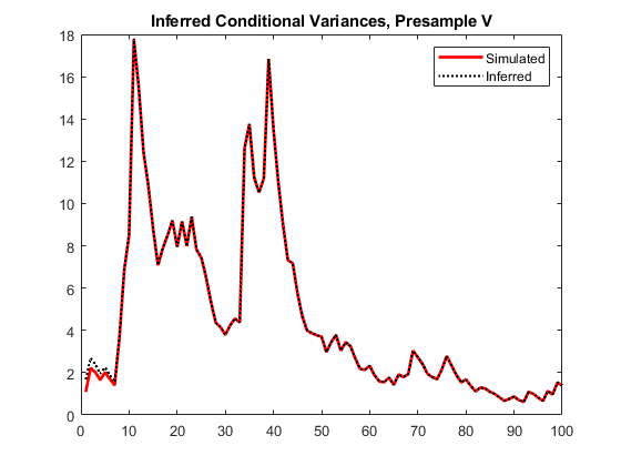
Infer conditional variances using the set-aside presample conditional variance, vO. Compare them to the known (simulated) conditional variances.

vO = infer(Mdl,y,V0=v0);

figure
plot(v)
plot(1:100,v,"r",LineWidth=2)
hold on
plot(1:100,vO,"k:",LineWidth=1.5)
legend("Simulated","Inferred",Location="northeast")
title("Inferred Conditional Variances, Presample V")
hold off

There is a much smaller transient response in the early time periods.

Infer conditional variances using both the presample innovation and conditional variance. Compare them to the known (simulated) conditional variances.

vEO = infer(Mdl,y,E0=y0,V0=v0);

figure
plot(v)
plot(1:100,v,"r",LineWidth=2)
hold on
plot(1:100,vEO,"k:",LineWidth=1.5)
legend("Simulated","Inferred",Location="northeast")
title("Inferred Conditional Variances, Presamples")
hold off

When you use sufficient presample innovations and conditional variances, the inferred conditional variances are exact (there is no transient response).

Conduct Likelihood Ratio Test for EGARCH Fit Comparison Specifying Data in Timetables

Since R2023a

Open Live Script

Infer the loglikelihood objective function values for an EGARCH(1,1) and EGARCH(2,1) model fit to the average weekly closing NASDAQ returns. To identify which model is the more parsimonious, adequate fit, conduct a likelihood ratio test. Specify data in timetables.

Load the U.S. equity indices data Data_EquityIdx.mat.

load Data_EquityIdx

The timetable DataTimeTable contains the daily NASDAQ closing prices, among other indices.

Compute the weekly average closing prices of all timetable variables.

DTTW = convert2weekly(DataTimeTable,Aggregation="mean");

Compute the weekly returns and their sample mean.

DTTRet = price2ret(DTTW);
DTTRet.Interval = [];
T = height(DTTRet)

T = 
626

When you plan to supply a timetable, you must ensure it has all the following characteristics:

The selected response variable is numeric and does not contain any missing values.
The timestamps in the Time variable are regular, and they are ascending or descending.

Remove all missing values from the timetable, relative to the NASDAQ returns series.

DTTRet = rmmissing(DTTRet,DataVariables="NASDAQ");
numobs = height(DTTRet)

numobs = 
626

Because all sample times have observed NASDAQ returns, rmmissing does not remove any observations.

Determine whether the sampling timestamps have a regular frequency and are sorted.

areTimestampsRegular = isregular(DTTRet,"weeks")

areTimestampsRegular = logical
   1

areTimestampsSorted = issorted(DTTRet.Time)

areTimestampsSorted = logical
   1

areTimestampsRegular = 1 indicates that the timestamps of DTTRet represent a regular weekly sample. areTimestampsSorted = 1 indicates that the timestamps are sorted.

Reserve the first two observations to use as a presample.

DTTRet0 = DTTRet(1:2,:);
DTTRet = DTTRet(3:end,:);

Fit an EGARCH(1,1) model to the returns. Supply in-sample and presample data in timetables, and specify NASDAQ as the variable containing the presample innovations. Infer the loglikelihood objective function value.

MdlEGARCH11 = egarch(1,1);
MdlEGARCH11.SeriesName = "NASDAQ";

EstMdlEGARCH11 = estimate(MdlEGARCH11,DTTRet, ...
    Presample=DTTRet0,PresampleInnovationVariable="NASDAQ");

 
    EGARCH(1,1) Conditional Variance Model (Gaussian Distribution):
 
                    Value      StandardError    TStatistic      PValue  
                   ________    _____________    __________    __________

    Constant       -0.48899       0.15218        -3.2133       0.0013123
    GARCH{1}        0.95567      0.013348         71.598               0
    ARCH{1}          0.2766      0.052276         5.2912      1.2154e-07
    Leverage{1}    -0.10593      0.025607        -4.1366      3.5244e-05

[TblEGARCH11,logLEGARCH11] = infer(EstMdlEGARCH11,DTTRet, ...
    Presample=DTTRet0,PresampleInnovationVariable="NASDAQ");
tail(TblEGARCH11)

       Time           NYSE          NASDAQ       NASDAQ_Variance    NASDAQ_Residual
    ___________    ___________    ___________    _______________    _______________

    16-Nov-2001      0.0021092      0.0048052      3.4439e-05           0.0048052  
    23-Nov-2001       0.001451     0.00085891      3.0717e-05          0.00085891  
    30-Nov-2001    -0.00039051      0.0020552      2.4587e-05           0.0020552  
    07-Dec-2001     0.00087108       0.005263      2.0775e-05            0.005263  
    14-Dec-2001      -0.002694     -0.0012244      2.0067e-05          -0.0012244  
    21-Dec-2001      0.0019929    -0.00094985      1.7698e-05         -0.00094985  
    28-Dec-2001      0.0019952      -4.93e-05      1.5413e-05           -4.93e-05  
    04-Jan-2002    -0.00011742     -0.0012263      1.2447e-05          -0.0012263

TblEGARCH11 is a timetable of NASDAQ residuals NASDAQ_Residual and conditional variances NASDAQ_Variance, and all variables in the specified in-sample data DTTRet. logLEGARCH11 is the loglikelihood of the estimated model EstMdlEGARCH11 evaluated at the specified presample and in-sample data.

Fit an EGARCH(2,1) model to the returns. Supply in-sample and presample data in timetables, and specify NASDAQ as the variable containing the presample innovations. Infer the loglikelihood objective function value.

MdlEGARCH21 = egarch(2,1);
MdlEGARCH21.SeriesName = "NASDAQ";

EstMdlEGARCH21 = estimate(MdlEGARCH21,DTTRet, ...
    Presample=DTTRet0,PresampleInnovationVariable="NASDAQ");

 
    EGARCH(2,1) Conditional Variance Model (Gaussian Distribution):
 
                     Value      StandardError    TStatistic      PValue  
                   _________    _____________    __________    __________

    Constant        -0.48641       0.15765         -3.0854       0.002033
    GARCH{1}         0.96882       0.27062            3.58     0.00034361
    GARCH{2}       -0.012906       0.26607       -0.048505        0.96131
    ARCH{1}          0.27422      0.074054          3.7029     0.00021312
    Leverage{1}     -0.10486      0.035239         -2.9756       0.002924

[TblEGARCH21,logLEGARCH21] = infer(EstMdlEGARCH21,DTTRet, ...
    Presample=DTTRet0,PresampleInnovationVariable="NASDAQ");

Conduct a likelihood ratio test, with the more parsimonious EGARCH(1,1) model as the null model, and the EGARCH(2,1) model as the alternative. The degree of freedom for the test is 1, because the EGARCH(2,1) model has one more parameter than the EGARCH(1,1) model (an additional GARCH term).

[h,p] = lratiotest(logLEGARCH21,logLEGARCH11,1)

h = logical
   0

p = 
0.9565

The null hypothesis is not rejected (h = 0). At the 0.05 significance level, the EGARCH(1,1) model is not rejected in favor of the EGARCH(2,1) model.

Conduct Likelihood Ratio Test for GARCH and GJR Fit Comparison

Open Live Script

A GARCH(P, Q) model is nested within a GJR(P, Q) model. Therefore, you can perform a likelihood ratio test to compare GARCH(P, Q) and GJR(P, Q) model fits.

Infer the loglikelihood objective function values for a GARCH(1,1) and GJR(1,1) model fit to NASDAQ Composite Index returns. Conduct a likelihood ratio test to identify which model is the more parsimonious, adequate fit.

Load the NASDAQ data included with the toolbox, and convert the index to returns. Set aside the first two observations to use as presample data.

load Data_EquityIdx
nasdaq = DataTable.NASDAQ;
r = price2ret(nasdaq);
r0 = r(1:2);
rn = r(3:end);

Fit a GARCH(1,1) model to the returns, and infer the loglikelihood objective function value.

Mdl1 = garch(1,1);
EstMdl1 = estimate(Mdl1,rn,E0=r0);

 
    GARCH(1,1) Conditional Variance Model (Gaussian Distribution):
 
                  Value       StandardError    TStatistic      PValue  
                __________    _____________    __________    __________

    Constant    2.0348e-06     5.4545e-07        3.7305       0.0001911
    GARCH{1}       0.88275       0.008499        103.87               0
    ARCH{1}        0.10956      0.0076979        14.233      5.7259e-46

[~,logL1] = infer(EstMdl1,rn,E0=r0);

Fit a GJR(1,1) model to the returns, and infer the loglikelihood objective function value.

Mdl2 = gjr(1,1);
EstMdl2 = estimate(Mdl2,rn,E0=r0);

 
    GJR(1,1) Conditional Variance Model (Gaussian Distribution):
 
                     Value       StandardError    TStatistic      PValue  
                   __________    _____________    __________    __________

    Constant       4.4478e-06     7.1366e-07        6.2325      4.5916e-10
    GARCH{1}           0.8064       0.013856        58.201               0
    ARCH{1}           0.11258       0.013474        8.3556      6.5084e-17
    Leverage{1}       0.11505       0.014367        8.0078      1.1678e-15

[~,logL2] = infer(EstMdl2,rn,E0=r0);

Conduct a likelihood ratio test, with the more parsimonious GARCH(1,1) model as the null model, and the GJR(1,1) model as the alternative. The degree of freedom for the test is 1, because the GJR(1,1) model has one more parameter than the GARCH(1,1) model (a leverage term).

[h,p] = lratiotest(logL2,logL1,1)

h = logical
   1

p = 
1.3606e-05

The null hypothesis is rejected (h = 1). At the 0.05 significance level, the GARCH(1,1) model is rejected in favor of the GJR(1,1) model.

Input Arguments

collapse all

`Mdl` — Conditional variance model
`garch` model object | `egarch` model object | `gjr` model object

Conditional variance model without any unknown parameters, specified as a garch, egarch, or gjr model object.

Mdl cannot contain any properties that have NaN value.

`Y` — Response data
numeric column vector | numeric matrix

Response data, specified as a numobs-by-1 numeric column vector or numobs-by-numpaths matrix.

As a column vector, Y represents a single path of the underlying series.

As a matrix, the rows of Y correspond to periods and the columns correspond to separate paths. The observations across any row occur simultaneously.

infer infers the conditional variances of Y. Y usually represents an innovation series with mean 0 and variances characterized by Mdl. It is the continuation of the presample innovation series E0. Y can also represent a time series of innovations with mean 0 plus an offset. If Mdl has a nonzero offset, then the software stores its value in the Offset property (Mdl.Offset).

The last observation of any series is the latest observation.

`Tbl1` — Time series data
table | timetable

Since R2023a

Time series data containing response variable y_t, at which infer evaluates the conditional variance model Mdl, specified as a table or timetable with numvars variables and numobs rows. You can optionally select a response variable by using the ResponseVariable name-value argument.

The selected variable is a single path (numobs-by-1 vector) or multiple paths (numobs-by-numpaths matrix) of numobs observations of response data. Each row is an observation, and measurements in each row occur simultaneously.

The selected response variable in Tbl1 is a numobs-by-numpaths numeric matrix. Each row is an observation, and measurements in each row occur simultaneously.

Each path (column) of the selected variable is independent of the other paths.

If Tbl1 is a timetable, it must represent a sample with a regular datetime time step (see isregular), and the datetime vector Tbl1.Time must be strictly ascending or descending.

If Tbl1 is a table, the last row contains the latest observation.

Name-Value Arguments

Specify optional pairs of arguments as Name1=Value1,...,NameN=ValueN, where Name is the argument name and Value is the corresponding value. Name-value arguments must appear after other arguments, but the order of the pairs does not matter.

Before R2021a, use commas to separate each name and value, and enclose Name in quotes.

Example: 'E0',[1 1;0.5 0.5],'V0',[1 0.5;1 0.5] specifies two equivalent presample paths of innovations and two, different presample paths of conditional variances.

`ResponseVariable` — Variable to select from `Tbl1` to treat as response variable y_t
string scalar | character vector | integer | logical vector

Since R2023a

Variable to select from Tbl1 to treat as the response variable y_t, specified as one of the following data types:

String scalar or character vector containing a variable name in Tbl1.Properties.VariableNames
Variable index (integer) to select from Tbl1.Properties.VariableNames
A length numvars logical vector, where ResponseVariable(j) = true selects variable j from Tbl1.Properties.VariableNames, and sum(ResponseVariable) is 1

The selected variable must be a numeric vector and cannot contain missing values (NaN).

If Tbl1 has one variable, the default specifies that variable. Otherwise, the default matches the variable to name in Mdl.SeriesName.

Example: ResponseVariable="StockRate2"

Example: ResponseVariable=[false false true false] or ResponseVariable=3 selects the third table variable as the response variable.

Data Types: double | logical | char | cell | string

`E0` — Presample innovation paths ε_t
numeric column vector | numeric matrix

Presample innovation paths ε_t, specified as a numpreobs-by-1 numeric column vector or a numpreobs-by-numprepaths matrix. The presample innovations provide initial values for the innovations process of the conditional variance model Mdl, and derive from a distribution with mean 0. Use E0 only when you supply the numeric array of response data Y.

numpreobs is the number of presample observations. numprepaths is the number of presample response paths.

Each row is a presample observation, and measurements in each row occur simultaneously. The last row contains the latest presample observation. numpreobs must be at least Mdl.Q. If numpreobs > Mdl.Q, infer uses the latest required number of observations only. The last element or row contains the latest observation.

If E0 is a column vector, it represents a single path of the underlying innovation series. infer applies it to each output path.
If E0 is a matrix, each column represents a presample path of the underlying innovation series. numprepaths must be at least numpaths. If numprepaths > numpaths, infer uses the first size(Y,2) columns only.

The defaults are:

For GARCH(P,Q) and GJR(P,Q) models, infer sets any necessary presample innovations to the square root of the average squared value of the offset-adjusted response series Y.
For EGARCH(P,Q) models, infer sets any necessary presample innovations to zero.

Data Types: double

`V0` — Positive presample conditional variance paths σ_t²
positive column vector | positive matrix

Positive presample conditional variance paths σ_t², specified as a numpreobs-by-1 positive column vector or numpreobs-by-numprepaths positive matrix. V0 provides initial values for the conditional variances in the model. Use V0 only when you supply the numeric array of disturbances Z.

Each row is a presample observation, and measurements in each row occur simultaneously. The last row contains the latest presample observation.

For GARCH(P,Q) and GJR(P,Q) models, numpreobs must be at least Mdl.P.
For EGARCH(P,Q) models,numpreobs must be at least max([Mdl.P Mdl.Q]).

numpreobs must be at least max([Mdl.P Mdl.Q]). If numpreobs > max([Mdl.P Mdl.Q]), infer uses the latest required number of observations only. The last element or row contains the latest observation.

If V0 is a column vector, it represents a single path of the conditional variance series. infer applies it to each output path.
If V0 is a matrix, each column represents a presample path of the conditional variance series. numprepaths must be at least numpaths. If numprepaths > numpaths, infer uses the first size(Y,2) columns only.

By default, infer sets any necessary presample conditional variances to the unconditional variance of the process.

Data Types: double

`Presample` — Presample data
table | timetable

Since R2023a

Presample data containing paths of innovation ε_t or conditional variance σ_t² series to initialize the model, specified as a table or timetable, the same type as Tbl1, with numprevars variables and numpreobs rows. Use Presample only when you supply a table or timetable of data Tbl1.

Each selected variable is a single path (numpreobs-by-1 vector) or multiple paths (numpreobs-by-numprepaths matrix) of numpreobs observations representing the presample of numpreobs observations of the innovation or conditional variance series for ResponseVariable, the selected response variable in Tbl1.

Each row is a presample observation, and measurements in each row occur simultaneously. numpreobs must be one of the following values:

Mdl.Q when Presample provides only presample innovations.
Mdl.P when Presample provides only presample conditional variances.
max([Mdl.P Mdl.Q]) when Presample provides both presample innovations and conditional variances

If numpreobs exceeds the minimum number, infer uses the latest required number of observations only.

If Presample is a timetable, all the following conditions must be true:

Presample must represent a sample with a regular datetime time step (see isregular).
The inputs Tbl1 and Presample must be consistent in time such that Presample immediately precedes Tbl1 with respect to the sampling frequency and order.
The datetime vector of sample timestamps Presample.Time must be ascending or descending.

If Presample is a table, the last row contains the latest presample observation.

The defaults are:

For GARCH(P,Q) and GJR(P,Q) models, infer sets any necessary presample innovations to the square root of the average squared value of the offset-adjusted response series Y.
For EGARCH(P,Q) models, infer sets any necessary presample innovations to zero.
infer sets any necessary presample conditional variances to the unconditional variance of the process.

If you specify the Presample, you must specify the presample innovation or conditional variance variable names by using the PresampleInnovationVariable or PresampleVarianceVariable name-value argument.

`PresampleInnovationVariable` — Variable of `Presample` containing presample innovation paths ε_t
string scalar | character vector | integer | logical vector

Since R2023a

Variable of Presample containing presample innovation paths ε_t, specified as one of the following data types:

String scalar or character vector containing a variable name in Presample.Properties.VariableNames
Variable index (integer) to select from Presample.Properties.VariableNames
A length numprevars logical vector, where PresampleInnovationVariable(j) = true selects variable j from Presample.Properties.VariableNames, and sum(PresampleInnovationVariable) is 1

The selected variable must be a numeric matrix and cannot contain missing values (NaN).

If you specify presample innovation data by using the Presample name-value argument, you must specify PresampleInnovationVariable.

Example: PresampleInnovationVariable="StockRateInnov0"

Example: PresampleInnovationVariable=[false false true false] or PresampleInnovationVariable=3 selects the third table variable as the presample innovation variable.

Data Types: double | logical | char | cell | string

`PresampleVarianceVariable` — Variable of `Presample` containing data for the presample conditional variances σ_t²
string scalar | character vector | integer | logical vector

Since R2023a

Variable of Presample containing data for the presample conditional variances σ_t², specified as one of the following data types:

String scalar or character vector containing a variable name in Presample.Properties.VariableNames
Variable index (positive integer) to select from Presample.Properties.VariableNames
A logical vector, where PresampleVarianceVariable(j) = true selects variable j from Presample.Properties.VariableNames

The selected variable must be a numeric vector and cannot contain missing values (NaNs).

If you specify presample conditional variance data by using the Presample name-value argument, you must specify PresampleVarianceVariable.

Example: PresampleVarianceVariable="StockRateVar0"

Example: PresampleVarianceVariable=[false false true false] or PresampleVarianceVariable=3 selects the third table variable as the presample conditional variance variable.

Data Types: double | logical | char | cell | string

Notes:

NaN values in Y, E0, and V0 indicate missing values. infer removes missing values from specified data by list-wise deletion.
- For the presample, infer horizontally concatenates E0 and V0, and then it removes any row of the concatenated matrix containing at least one NaN.
- For in-sample data Y, infer removes any row containing at least one NaN.
This type of data reduction reduces the effective sample size and can create an irregular time series.
For numeric data inputs, infer assumes that you synchronize the presample data such that the latest observations occur simultaneously.
infer issues an error when any table or timetable input contains missing values.

Output Arguments

collapse all

`V` — Conditional variances
numeric column vector | numeric matrix

Conditional variances inferred from the response data Y, returned as a numeric column vector or matrix. infer returns V only when you supply the input Y.

The dimensions of V and Y are equivalent. If Y is a matrix, then the columns of V are the inferred conditional variance paths corresponding to the columns of Y.

Rows of V are periods corresponding to the periodicity of Y.

`logL` — Loglikelihood objective function values
numeric scalar | numeric vector

Loglikelihood objective function values associated with the model Mdl, returned as a numeric scalar or vector of length numpaths.

If Y is a vector, then logL is a scalar. Otherwise, logL is vector of length size(Y,2), and each element is the loglikelihood of the corresponding column (or path) in Y.

`Tbl2` — Inferred conditional variance σ_t² and innovation ε_t paths
table | timetable

Since R2023b

Inferred conditional variance σ_t² and innovation ε_t paths, returned as a table or timetable, the same data type as Tbl1. infer returns Tbl2 only when you supply the input Tbl1. When Mdl is an estimated model returned by estimate, the returned, inferred innovations are residuals.

Tbl2 contains the following variables:

The inferred conditional variance paths, which are in a numobs-by-numpaths numeric matrix, with rows representing observations and columns representing independent paths. Each path represents the continuation of the corresponding path of presample conditional variances in Presample. infer names the filtered conditional variance variable in Tbl2 responseName_Variance, where responseName is Mdl.SeriesName. For example, if Mdl.SeriesName is StockReturns, Tbl2 contains a variable for the corresponding inferred conditional variance paths with the name StockReturns_Variance.
The inferred innovation paths, which are in a numobs-by-numpaths numeric matrix, with rows representing observations and columns representing independent paths. Each path corresponds to the input response path in Tbl1 and represents the continuation of the corresponding presample innovations path in Presample. infer names the inferred innovations variable in Tbl2 responseName_Residual, where responseName is Mdl.SeriesName. For example, if Mdl.SeriesName is StockReturns, Tbl2 contains a variable for the corresponding inferred innovations paths with the name StockReturns_Residual.
All variables Tbl1.

If Tbl1 is a timetable, row times of Tbl1 and Tbl2 are equal.

Algorithms

If you do not specify presample data (E0 and V0, or Presample), infer derives the necessary presample observations from the unconditional, or long-run, variance of the offset-adjusted response process.

For all conditional variance model types, required presample conditional variances are the sample average of the squared disturbances of the offset-adjusted specified response data (Y or Tbl1).
For GARCH(P,Q) and GJR(P,Q) models, the required presample innovations are the square root of the average squared value of the offset-adjusted response data.
For EGARCH(P,Q) models, the required presample innovaitons are 0.

These specifications minimize initial transient effects.

References

[1] Bollerslev, T. “Generalized Autoregressive Conditional Heteroskedasticity.” Journal of Econometrics. Vol. 31, 1986, pp. 307–327.

[2] Bollerslev, T. “A Conditionally Heteroskedastic Time Series Model for Speculative Prices and Rates of Return.” The Review of Economics and Statistics. Vol. 69, 1987, pp. 542–547.

[3] Box, G. E. P., G. M. Jenkins, and G. C. Reinsel. Time Series Analysis: Forecasting and Control. 3rd ed. Englewood Cliffs, NJ: Prentice Hall, 1994.

[4] Enders, W. Applied Econometric Time Series. Hoboken, NJ: John Wiley & Sons, 1995.

[5] Engle, R. F. “Autoregressive Conditional Heteroskedasticity with Estimates of the Variance of United Kingdom Inflation.” Econometrica. Vol. 50, 1982, pp. 987–1007.

[6] Glosten, L. R., R. Jagannathan, and D. E. Runkle. “On the Relation between the Expected Value and the Volatility of the Nominal Excess Return on Stocks.” The Journal of Finance. Vol. 48, No. 5, 1993, pp. 1779–1801.

[7] Hamilton, J. D. Time Series Analysis. Princeton, NJ: Princeton University Press, 1994.

Version History

Introduced in R2012a

expand all

R2023a: `infer` accepts input data in tables and timetables, and returns results in tables and timetables

In addition to accepting input data (in-sample and presample) in numeric arrays, infer accepts input data in tables or regular timetables. When you supply data in a table or timetable, the following conditions apply:

infer chooses the default in-sample response series on which to operate, but you can use the specified optional name-value argument to select a different series.
If you specify optional presample innovation or conditional variance data to initialize the model, you must also specify the presample innovation or conditional variance series name.
infer returns results in a table or timetable.

Name-value arguments to support tabular workflows include:

ResponseVariable specifies the variable name of the response paths in the input data, from which infer infers conditional variances and innovations.
Presample specifies the input table or timetable of presample innovation and conditional variance data.
PresampleInnovationVariable specifies the variable name of the innovation paths to select from Presample.
PresampleVarianceVariable specifies the variable name of the conditional variance paths to select from Presample.

infer

Syntax

Description

Examples

Infer GARCH Model Conditional Variances From Numeric Response Data

Infer EGARCH Model Conditional Variances

Infer GJR Model Conditional Variances

Conduct Likelihood Ratio Test for EGARCH Fit Comparison Specifying Data in Timetables

Conduct Likelihood Ratio Test for GARCH and GJR Fit Comparison

Input Arguments

`Mdl` — Conditional variance model
`garch` model object | `egarch` model object | `gjr` model object

`Y` — Response data
numeric column vector | numeric matrix

`Tbl1` — Time series data
table | timetable

Name-Value Arguments

`ResponseVariable` — Variable to select from `Tbl1` to treat as response variable y_t
string scalar | character vector | integer | logical vector

`E0` — Presample innovation paths ε_t
numeric column vector | numeric matrix

`V0` — Positive presample conditional variance paths σ_t²
positive column vector | positive matrix

`Presample` — Presample data
table | timetable

`PresampleInnovationVariable` — Variable of `Presample` containing presample innovation paths ε_t
string scalar | character vector | integer | logical vector

`PresampleVarianceVariable` — Variable of `Presample` containing data for the presample conditional variances σ_t²
string scalar | character vector | integer | logical vector

Output Arguments

`V` — Conditional variances
numeric column vector | numeric matrix

`logL` — Loglikelihood objective function values
numeric scalar | numeric vector

`Tbl2` — Inferred conditional variance σ_t² and innovation ε_t paths
table | timetable

Algorithms

References

Version History

R2023a: `infer` accepts input data in tables and timetables, and returns results in tables and timetables

See Also

Objects

Functions

Topics

infer

Syntax

Description

Examples

Infer GARCH Model Conditional Variances From Numeric Response Data

Infer EGARCH Model Conditional Variances

Infer GJR Model Conditional Variances

Conduct Likelihood Ratio Test for EGARCH Fit Comparison Specifying Data in Timetables

Conduct Likelihood Ratio Test for GARCH and GJR Fit Comparison

Input Arguments

Mdl — Conditional variance model garch model object | egarch model object | gjr model object

Y — Response data numeric column vector | numeric matrix

Tbl1 — Time series data table | timetable

Name-Value Arguments

ResponseVariable — Variable to select from Tbl1 to treat as response variable yt string scalar | character vector | integer | logical vector

E0 — Presample innovation paths εt numeric column vector | numeric matrix

V0 — Positive presample conditional variance paths σt2 positive column vector | positive matrix

Presample — Presample data table | timetable

PresampleInnovationVariable — Variable of Presample containing presample innovation paths εt string scalar | character vector | integer | logical vector

PresampleVarianceVariable — Variable of Presample containing data for the presample conditional variances σt2 string scalar | character vector | integer | logical vector

Output Arguments

V — Conditional variances numeric column vector | numeric matrix

logL — Loglikelihood objective function values numeric scalar | numeric vector

Tbl2 — Inferred conditional variance σt2 and innovation εt paths table | timetable

Algorithms

References

Version History

R2023a: infer accepts input data in tables and timetables, and returns results in tables and timetables

See Also

Objects

Functions

Topics

`Mdl` — Conditional variance model
`garch` model object | `egarch` model object | `gjr` model object

`Y` — Response data
numeric column vector | numeric matrix

`Tbl1` — Time series data
table | timetable

`ResponseVariable` — Variable to select from `Tbl1` to treat as response variable y_t
string scalar | character vector | integer | logical vector

`E0` — Presample innovation paths ε_t
numeric column vector | numeric matrix

`V0` — Positive presample conditional variance paths σ_t²
positive column vector | positive matrix

`Presample` — Presample data
table | timetable

`PresampleInnovationVariable` — Variable of `Presample` containing presample innovation paths ε_t
string scalar | character vector | integer | logical vector

`PresampleVarianceVariable` — Variable of `Presample` containing data for the presample conditional variances σ_t²
string scalar | character vector | integer | logical vector

`V` — Conditional variances
numeric column vector | numeric matrix

`logL` — Loglikelihood objective function values
numeric scalar | numeric vector

`Tbl2` — Inferred conditional variance σ_t² and innovation ε_t paths
table | timetable

R2023a: `infer` accepts input data in tables and timetables, and returns results in tables and timetables