PanelModel

Panel data regression model

Since R2026a

Description

PanelModel is an object that encapsulates a fitted panel (longitudinal) data regression model. A panel data regression model describes the linear relationship between a response variable and predictor variables, in which the data set is a random, observational sample of n subjects measured over T time points. The model accommodates a linear random effect (heterogeneity), which you can use to control for, and study, unobserved, subject-specific, phenomena associated with the response variable.

Use the properties of a PanelData object to investigate the fitted panel data regression model. The object properties include information about coefficient and effect estimates, associated variances and covariances, and inferences.

Creation

Create a PanelModel object by using the fitrepanel function.

fitrepanel fits a random effects panel data regression model to data. That is, the observed and unobserved effects are independent (not to be confused with the random effects of a linear mixed-effects model, as computed by the fitlme function).

Properties

expand all

`Coefficients` — Regression coefficient estimates β
numeric vector

Regression coefficient estimates β associated with the predictor variables x, stored as a p-by-1 numeric vector.

Data Types: double

`CoefficientCovariance` — Estimated covariance matrix of regression coefficient estimates Σ
numeric matrix

Estimated covariance matrix of regression coefficient estimates Σ, stored as a p-by-p numeric matrix.

Data Types: double

`DisturbanceVariance` — Model disturbance variance estimate σ²_ε
nonnegative numeric scalar

Model disturbance variance estimate σ²_ε, stored as a nonnegative numeric scalar. If you specify DisturbanceVariance when you call fitrepanel, DisturbanceVariance stores the specification.

Data Types: double

`EffectVariance` — Effect variance estimate σ²_ɑ
nonnegative numeric scalar

Effect variance estimate σ²_ɑ, stored as a nonnegative numeric scalar. If you specify EffectVariance when you call fitrepanel, EffectVariance stores the specification.

Data Types: double

`Effects` — Estimated effects ɑ, or heterogeneity
numeric vector | `[]`

Estimated effects ɑ, or heterogeneity, stored as an n-by-1 numeric vector. If you specify FitEffects=false when you call fitrepanel, Effects is an empty array ([]).

Data Types: double

`Loglikelihood` — Loglikelihood
numeric scalar

Loglikelihood associated with the fitted model and data, stored as a numeric scalar.

Data Types: double

`Summary` — Statistical estimation summary
table

Statistical estimation summary, stored as a table.

Data Types: double

`Type` — Panel data regression model type
`"RandomEffects"`

Panel data regression model type, stored as "RandomEffects".

Data Types: string

Examples

collapse all

Fit Random Effects Panel Regression Model to Data in Wide Format

Open Live Script

Fit a random effects panel data regression model to data using default options. The data is in wide format.

Load the simulated, balanced panel data set Data_SimulatedBalancedPanel.mat, which is available when you open this example. The data set contains 12 microeconomic measurements of 1000 randomly selected people taken yearly from 2006 through 2020. The response variable in the model is a series of log wages, while all other variables in the data are predictors.

load Data_SimulatedBalancedPanel

For details on the data set, enter Description at the command line.

The variable Data is a 3-D numeric array containing the predictor and response variables. Each row is a time point in the sampling period, each column is a subject in the sample, and each page is a variable. The final variable in Data is the response variable (log wages series), while all other variables are predictors.

Create separate variables for the predictor and response data.

X = Data(:,:,1:(end-1));
Y = Data(:,:,end);

X is a 15-by-1000-by-11 numeric array of predictor data and Y is a 15-by-1000 numeric matrix. For example, X(10,501,3) is the education experience of subject 501 in 2015.

Create a binary numeric variable for whether the subject is female (coded as 1), by using predictor 2, and a binary numeric variable for whether the subject is married (coded as 1), by using predictor 9.

X(:,:,2) = double(X(:,:,2) == 1);
X(:,:,9) = double(X(:,:,9) == 1);

Assume that the subject effect (heterogeneity) is not associated with the predictor variables. Fit a random effects panel data regression model to the data. Use default options.

EstMdl = fitrepanel(X,Y);

Panel data information: 
Number of cross-sectional units (N):  1000
Number of periods (T):  15
Number of observations:  15000
Method of estimation:  random effects (GLS)

                     | Estimator    SE      tStat   pValue 
-----------------------------------------------------------
 x1                  |   0.0485   0.0003  154.4327   0     
 x2                  |  -0.3381   0.0324  -10.4265  0.0000 
 x3                  |   0.1003   0.0036   28.0246  0.0000 
 x4                  |  -0.1370   0.0389   -3.5231  0.0004 
 x5                  |  -0.0620   0.0047  -13.1530  0.0000 
 x6                  |   0.0087   0.0053    1.6637  0.0962 
 x7                  |  -0.0390   0.0112   -3.4902  0.0005 
 x8                  |  -0.0191   0.0071   -2.6853  0.0072 
 x9                  |  -0.0516   0.0107   -4.8406  0.0000 
 x10                 |   0.0741   0.0051   14.6575  0.0000 
 x11                 |   0.0016   0.0003    5.7319  0.0000 
 DisturbanceVariance |   0.0302                            
 EffectVariance      |   0.0947

fitrepanel displays an estimation summary to the command line. Row xj contains, for predictor j, the coefficient estimate, standard error, and $t$ statistic for a two-tailed $t$ test that the coefficient is 0 with its $p$ -value. All predictor variables are significant except for x6 and x7.

Display the fitted model.

EstMdl

EstMdl = 
  PanelModel with properties:

             Coefficients: [11×1 double]
    CoefficientCovariance: [11×11 double]
      DisturbanceVariance: 0.0302
           EffectVariance: 0.0947
                  Effects: [4.5484 4.3304 4.6605 4.9304 4.9176 4.5704 3.8183 4.7566 4.4485 4.1725 4.6417 4.5086 4.7519 4.4794 4.2617 4.7618 4.5002 4.3778 4.1206 3.8693 3.9290 4.5513 4.5366 4.2080 4.6091 4.2711 4.6690 3.7448 3.9863 … ] (1×1000 double)
            LogLikelihood: 4.9624e+03
                  Summary: [13×4 table]
                     Type: "RandomEffects"

EstMdl is a PanelModel object. You can access its properties using dot notation.

Plot the empirical distribution of the heterogeneity.

effects = EstMdl.Effects;
histogram(effects,Normalization="probability")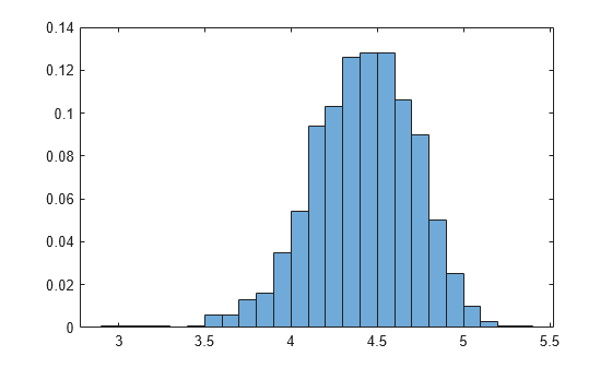

Figure contains an axes object. The axes object contains an object of type histogram.

Obtain Robust Estimates From Random Effects Panel Regression

Open Live Script

Fit a random effects panel data regression model to data and obtain robust estimates.

load Data_SimulatedBalancedPanel

For details on the data set, enter Description at the command line.

Create separate variables for the predictor and response data.

X = Data(:,:,1:(end-1));
[T,n,p] = size(X);
Y = Data(:,:,end);

X(:,:,2) = double(X(:,:,2) == 1);
X(:,:,9) = double(X(:,:,9) == 1);

Simulate heteroscedasticity in the system by using unmeasured, subject-specific predictor variables $z_{j}$ such that, for each subject $j = 1, . . ., n$ , $z_{j} \sim P o i s (λ_{j})$ and $λ_{j} \sim U n i f o r m (1, . . ., 50)$ . For each subject, simulate $T$ values.

rng(1,"twister")
Z = zeros(T,n);
for j = 1:n
    lambda = randi(50);
    Z(:,j) = poissrnd(lambda,T,1);
end

Add the simulated predictor data to the response data with coefficient $β_{z} = 2$ .

YSim = Y + 2*Z;

Assume that the heterogeneity is not associated with the predictor variables. Fit a random effects panel data regression model to the predictor data without $z$ and the simulated response data. Use default options.

EstMdl = fitrepanel(X,YSim);

Panel data information: 
Number of cross-sectional units (N):  1000
Number of periods (T):  15
Number of observations:  15000
Method of estimation:  random effects (GLS)

                     | Estimator    SE     tStat   pValue 
----------------------------------------------------------
 x1                  |    0.0196  0.0190   1.0279  0.3040 
 x2                  |    1.4279  3.0659   0.4657  0.6414 
 x3                  |   -0.1095  0.3385  -0.3236  0.7462 
 x4                  |   -2.0201  3.6775  -0.5493  0.5828 
 x5                  |    0.3700  0.2763   1.3392  0.1805 
 x6                  |   -0.2306  0.3087  -0.7472  0.4550 
 x7                  |    0.9527  0.6997   1.3616  0.1733 
 x8                  |    0.1847  0.4256   0.4341  0.6642 
 x9                  |    0.3463  0.6632   0.5223  0.6015 
 x10                 |   -0.0337  0.2965  -0.1137  0.9094 
 x11                 |    0.0070  0.0161   0.4345  0.6640 
 DisturbanceVariance |  101.9401                          
 EffectVariance      |  859.3624

Compute model residuals ${ε_{}^{ˆ}}_{t i} = Y_{t i} - X_{t i} β_{}^{ˆ} - {α_{}^{ˆ}}_{i}$ , and plot them against the fitted responses. Color the residuals according to subject ID.

betahat = reshape(EstMdl.Coefficients,1,1,p);
alphahat = EstMdl.Effects;
Yhat = sum(X.*betahat,3) + alphahat;
Residuals = YSim - Yhat;
figure
plot(Yhat,Residuals,'.')
hold on
yline(0,"--")
hold off
title("Residuals by Subject")
ylabel("Residual")
xlabel("Fitted Value")

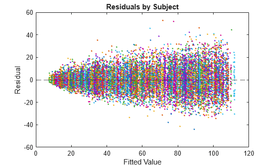
Figure contains an axes object. The axes object with title Residuals by Subject, xlabel Fitted Value, ylabel Residual contains 1001 objects of type line, constantline.

The residuals scatter more widely as the fitted values increase. This behavior is indicative of heteroscedasticity. Also, residuals appear clustered by groups.

Refit the model; compute robust covariance estimates.

EstMdlRobust = fitrepanel(X,YSim,RobustCovariance=true);

Panel data information: 
Number of cross-sectional units (N):  1000
Number of periods (T):  15
Number of observations:  15000
Method of estimation:  random effects (GLS)

                     | Estimator    SE     tStat   pValue 
----------------------------------------------------------
 x1                  |    0.0196  0.0191   1.0222  0.3067 
 x2                  |    1.4279  2.8975   0.4928  0.6222 
 x3                  |   -0.1095  0.3417  -0.3205  0.7486 
 x4                  |   -2.0201  3.5807  -0.5642  0.5726 
 x5                  |    0.3700  0.2755   1.3431  0.1792 
 x6                  |   -0.2306  0.3215  -0.7174  0.4731 
 x7                  |    0.9527  0.6701   1.4218  0.1551 
 x8                  |    0.1847  0.4344   0.4253  0.6706 
 x9                  |    0.3463  0.6501   0.5327  0.5942 
 x10                 |   -0.0337  0.2976  -0.1133  0.9098 
 x11                 |    0.0070  0.0159   0.4414  0.6589 
 DisturbanceVariance |  101.9401                          
 EffectVariance      |  859.3624

The coefficient estimates between the regular and robust runs are the same; the difference between the runs is in the inferences.

Plot a heatmap of the difference between the estimated coefficient covariance matrix.

seriesSim = series(1:p);
heatmap(seriesSim,seriesSim,(EstMdlRobust.CoefficientCovariance-EstMdl.CoefficientCovariance)./EstMdl.CoefficientCovariance)

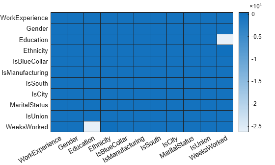
Figure contains an object of type heatmap.

The estimated covariance of the coefficients of Education and WeeksWorked shows the greatest relative difference between the robust and non-robust analyses.

Alternative Functionality

When your longitudinal data set is the result of a controlled experiment study, fit a linear mixed-effects model (LinearMixedModel object) by using fitlme.

References

[1] Wooldridge, Jeffrey M. Econometric Analysis of Cross Section and Panel Data, Second edition. Cambridge, MA: The MIT Press, 2010.

[2] Greene, William H. Econometric Analysis, Fifth edition. New York: Pearson, 2018.

Version History

Introduced in R2026a

PanelModel

Description

Creation

Properties

Coefficients — Regression coefficient estimates β numeric vector

CoefficientCovariance — Estimated covariance matrix of regression coefficient estimates Σ numeric matrix

DisturbanceVariance — Model disturbance variance estimate σ2ε nonnegative numeric scalar

EffectVariance — Effect variance estimate σ2ɑ nonnegative numeric scalar

Effects — Estimated effects ɑ, or heterogeneity numeric vector | []

Loglikelihood — Loglikelihood numeric scalar

Summary — Statistical estimation summary table

Type — Panel data regression model type "RandomEffects"

Examples

Fit Random Effects Panel Regression Model to Data in Wide Format

Obtain Robust Estimates From Random Effects Panel Regression

Alternative Functionality

References

Version History

See Also

`Coefficients` — Regression coefficient estimates β
numeric vector

`CoefficientCovariance` — Estimated covariance matrix of regression coefficient estimates Σ
numeric matrix

`DisturbanceVariance` — Model disturbance variance estimate σ²_ε
nonnegative numeric scalar

`EffectVariance` — Effect variance estimate σ²_ɑ
nonnegative numeric scalar

`Effects` — Estimated effects ɑ, or heterogeneity
numeric vector | `[]`

`Loglikelihood` — Loglikelihood
numeric scalar

`Summary` — Statistical estimation summary
table

`Type` — Panel data regression model type
`"RandomEffects"`