Perform ARIMA Model Residual Diagnostics Using Econometric Modeler App

This example shows how to evaluate ARIMA model assumptions by performing residual diagnostics in the Econometric Modeler app. The data set, which is stored in Data_JAustralian.mat, contains the log quarterly Australian Consumer Price Index (CPI) measured from 1972 and 1991, among other time series.

Import Data into Econometric Modeler

At the command line, load the Data_JAustralian.mat data set.

load Data_JAustralian

At the command line, open the Econometric Modeler app.

econometricModeler

Alternatively, open the app from the apps gallery (see Econometric Modeler).

Import DataTimeTable into the app:

On the Econometric Modeler tab, in the Import section, click the Import button .
In the Import Data dialog box, in the Import? column, select the check box for the DataTimeTable variable.
Click Import.

The variables, including PAU, appear in the Time Series pane, and a time series plot containing all the series appears in the Time Series Plot(EXCH) figure window.

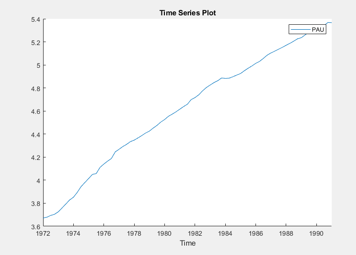
Create a time series plot of PAU by double-clicking PAU in the Time Series pane.

This screen shot shows a time series plot of the variable PAU where the x axis shows a time period from 1972 through the early 1990's.

Specify and Estimate ARIMA Model

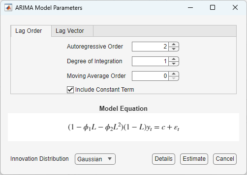
Estimate an ARIMA(2,1,0) model for the log quarterly Australian CPI (for details, see Implement Box-Jenkins Model Selection and Estimation Using Econometric Modeler App).

In the Time Series pane, select the PAU time series.
On the Econometric Modeler tab, in the Models section, click ARIMA.
In the ARIMA Model Parameters dialog box, on the Lag Order tab:
1. Set the Degree of Integration to 1.
2. Set the Autoregressive Order to 2.
Click Estimate.

The model variable ARIMA_PAU appears in the Models pane, its value appears in the Preview pane, and its estimation summary appears in the Model Summary(ARIMA_PAU) document.

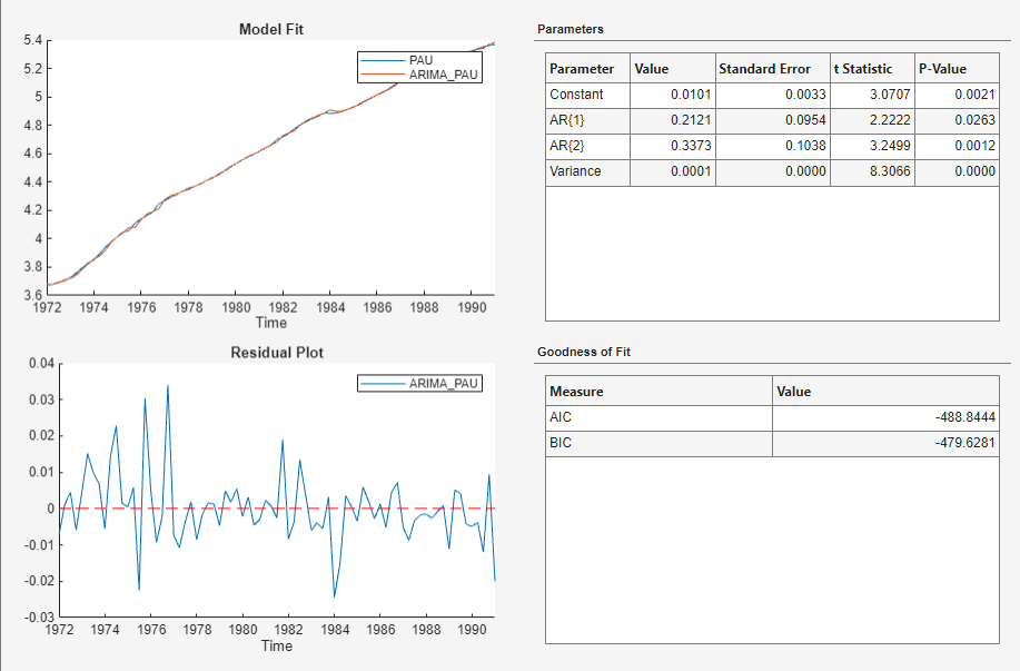
Model Summary (ARIMA_PAU) tab shows time series plots of Model Fit and Residual Plot. To the right are two tables, one for Parameters on top and one for Goodness of Fit below.

In the Model Summary(ARIMA_PAU) document, the Residual Plot figure is a time series plot of the residuals. The plot suggests that the residuals are centered at y = 0 and they exhibit volatility clustering.

Perform Residual Diagnostics

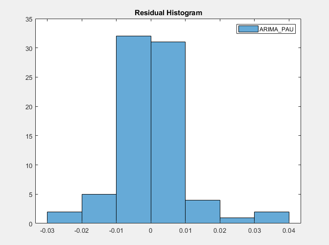
Visually assess whether the residuals are normally distributed by plotting their histogram and a quantile-quantile plot:

Close the Model Summary(ARIMA_PAU) document.
With ARIMA_PAU selected in the Models pane, on the Econometric Modeler tab, in the Diagnostics section, click Residual Diagnostics > Residual Histogram.
Click Residual Diagnostics > Residual Q-Q Plot.

Inspect the histogram by clicking the Histogram(ARIMA_PAU) figure window.

A screen shot of the Residual Histogram for ARIMA_PAU shown as a bar chart.

Inspect the quantile-quantile plot by clicking the QQPlot(ARIMA_PAU) figure window.

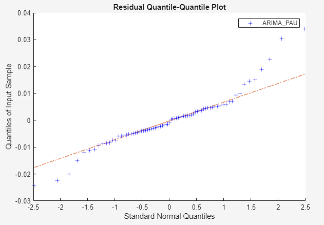
A screen shot of the Residual Quantile-Quantile Plot for ARIMA_PAU with Quantities of Input Sample shown on the y axis and Standard Normal Quantiles represented on the x axis.

The residuals appear approximately normally distributed. However, there is an excess of large residuals, which indicates that a t innovation distribution might be a reasonable model modification.

Visually assess whether the residuals are serially correlated by plotting their autocorrelations. With ARIMA_PAU selected in the Models pane, in the Diagnostics section, click Residual Diagnostics > Autocorrelation Function.

A time series plot of the Residual Sample Autocorrelation Function for ARIMA_PAU with Sample Autocorrelation shown on the y axis and Lag represented on the x axis. Confidence bounds are represented by blue horizontal lines.

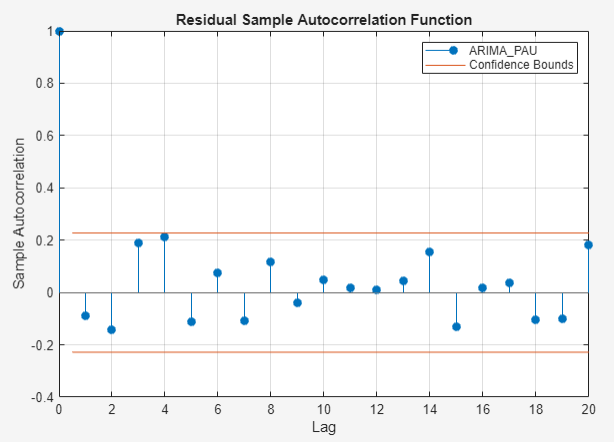
All lags that are greater than 0 correspond to insignificant autocorrelations. Therefore, the residuals are uncorrelated in time.

Visually assess whether the residuals exhibit heteroscedasticity by plotting the ACF of the squared residuals. With ARIMA_PAU selected in the Models pane, click the Econometric Modeler tab. Then, click the Diagnostics section, click Residual Diagnostics > Squared Residual Autocorrelation.

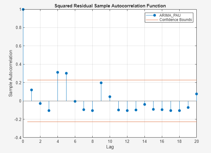
A time series plot of the Squared Residual Sample Autocorrelation Function for ARIMA_PAU with Sample Autocorrelation shown on the y axis and Lag represented on the x axis. Confidence bounds are represented by blue horizontal lines.

Significant autocorrelations occur at lags 4 and 5, which suggests a composite conditional mean and variance model for PAU.