Rolling-Window Analysis of Time-Series Models
Rolling-window analysis of a time-series model assesses:
The stability of the model over time. A common time-series model assumption is that the coefficients are constant with respect to time. Checking for instability amounts to examining whether the coefficients are time-invariant.
The forecast accuracy of the model.
Rolling-Window Analysis for Parameter Stability
Suppose that you have data for all periods in the sample. To check the stability of a time-series model using a rolling window:
Choose a rolling window size, m, i.e., the number of consecutive observation per rolling window. The size of the rolling window will depend on the sample size, T, and periodicity of the data. In general, you can use a short rolling window size for data collected in short intervals, and a larger size for data collected in longer intervals. Longer rolling window sizes tend to yield smoother rolling window estimates than shorter sizes.
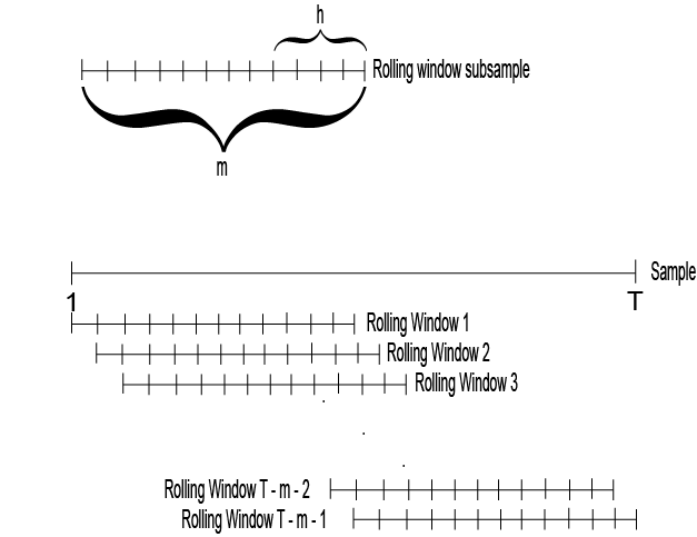
Suppose that the number of increments between successive rolling windows is 1 period, then partition the entire data set into N = T – m + 1 subsamples. The first rolling window contains observations for period 1 through m, the second rolling window contains observations for period 2 through m + 1, and so on.
There are variations on the partitions, e.g., rather than roll one observation ahead, you can roll four observations for quarterly data.
Estimate the model using each rolling window subsamples.
Plot each estimate and point-wise confidence intervals (i.e., ) over the rolling window index to see how the estimate changes with time. You should expect a little fluctuation for each, but large fluctuations or trends indicate that the parameter might be time varying.
For more details on assessing the stability of a model using rolling window analysis, see [1].
Rolling Window Analysis for Predictive Performance
Suppose that you have data for all periods in the sample. You can backtest to check the predictive performance of several time-series models using a rolling window. These steps outline how to backtest.
Choose a rolling window size, m, i.e., the number of consecutive observation per rolling window. The size of the rolling window depends on the sample size, T, and periodicity of the data. In general, you can use a short rolling window size for data collected in short intervals, and a larger size for data collected in longer intervals. Longer rolling window sizes tend to yield smoother rolling window estimates than shorter sizes.
Choose a forecast horizon, h. The forecast horizon depends on the application and periodicity of the data. The following illustrates how the rolling window partitions the data set.
If the number of increments between successive rolling windows is 1 period, then partition the entire data set into N = T – m + 1 subsamples. The first rolling window contains observations for period 1 through m, the second rolling window contains observations for period 2 through m + 1, and so on. The figure illustrates the partitions.

There are variations on the partitions, e.g., rather than roll one observation ahead, you can roll four observations for quarterly data.
For each rolling window subsample:
Estimate each model.
Estimate h-step-ahead forecasts.
Compute the forecast errors for each forecast, that is , where:
enj is the forecast error of rolling window n for the j-step-ahead forecast.
y is the response.
is the j-step-ahead forecast of rolling window subsample n.
Compute the root forecast mean squared errors (RMSEs) using the forecast errors for each step-ahead forecast type. In other words,
Compare the RMSEs among the models. The model with the lowest set of RMSEs has the best predictive performance.
For more details on backtesting, see [1].
References
[1] Zivot, E., and J. Wang. Modeling Financial Time Series with S_PLUS®. 2nd ed. NY: Springer Science+Business Media, Inc., 2006.