Specifying Univariate Lag Operator Polynomials Interactively
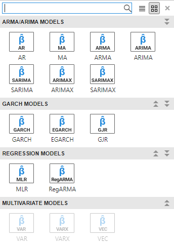
Consider building a predictive, univariate time series model (conditional mean, conditional variance, or regression model with ARMA errors) by using the Econometric Modeler app. After you choose candidate models for estimation (see Perform Exploratory Data Analysis), you can specify the model structure of each. To do so, on the Modeler tab, in the Models section, click a model or display the gallery of supported models and click the model you want.
After you select a time series model, the Type Model
Parameters dialog box appears, where Type is the model type.
For example, if you select SARIMAX, then the SARIMAX Model
Parameters dialog box appears.
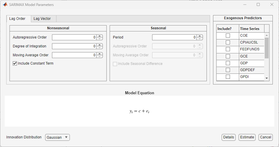
For all dynamic models, Econometric Modeler supports two options to specify the lag operator polynomials. The adjustment options are on separate tabs: the Lag Order and Lag Vector tab. The Lag Order tab options offer a straight forward way to include consecutive lags from lag 1 and degrees of integration (see Specify Lag Structure Using Lag Order Tab). The Lag Vector tab options allow you to create flexible models (see Specify Lag Structure Using Lag Vector Tab).
The
TypeModel Parameters dialog box contains a Nonseasonal or Seasonal section. The Seasonal section is absent in strictly nonseasonal model dialog boxes. To specify the nonseasonal lag operator polynomial structure, use the parameters in the Nonseasonal section. To adjust the seasonal lag operator polynomial structure, including seasonality, use the parameters in the Seasonal section.To specify the degrees of nonseasonal integration, in the Nonseasonal section, in the Degree of Integration (D) box, type the degree, or click the appropriate arrow on
 . You can specify up to 2 degrees of
nonseasonal integration.
. You can specify up to 2 degrees of
nonseasonal integration.To specify the seasonal periodicity for seasonal models, in the Seasonal section, in the Seasonality (s) box, type the periodicity, or click the appropriate arrow on
. When the periodicity is greater than 0,
you can specify the seasonal autoregressive or moving average polynomial
order, and you can specify up to one degree of seasonal integration. For verification, the model form appears in the Model Equation section. The model form updates to your specifications in real time.
Specify Lag Structure Using Lag Order Tab
On the Lag Order tab, in the Nonseasonal
section, you can specify the orders of each lag operator polynomial in the
nonseasonal component. In the appropriate lag polynomial order box (for example, the
Autoregressive Order (p) box), type
the nonnegative integer order or click the appropriate arrow on
![]() . The app includes all consecutive lags from 1
through
. The app includes all consecutive lags from 1
through LL
For seasonal models, on the Lag Order tab, in the Seasonal section:
Specify the period in the season by entering the nonnegative integer period in the Seasonality box or by clicking
.Specify the seasonal lag operator polynomial order. In the appropriate lag polynomial order box (for example, the Autoregressive Order (ps) box), type the nonnegative integer order ignoring seasonality or click
. The lag operator exponents in the
resulting polynomial are multiples of the specified period.
For example, in the Seasonal section, if
Seasonality is 4 and
Autoregressive Order
(ps) is
3, the seasonal autoregressive polynomial is .
You can specify up to one degree of seasonal integration by typing it into the
Degree of Integration
(Ds) box or clicking
![]() . When you specify one degree of seasonal
integration, a seasonal difference polynomial appears in the Model
Equation section, and its lag operator exponent is equal to the
specified period.
. When you specify one degree of seasonal
integration, a seasonal difference polynomial appears in the Model
Equation section, and its lag operator exponent is equal to the
specified period.
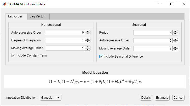
Consider a SARIMA(0,1,1)×(0,1,2)4 model, a seasonal multiplicative ARIMA model with four periods in a season (e.g., quarterly data). To specify this model using the parameters in the Lag Order tab:
Select a time series variable in the Time Series pane.
On the Modeler tab, in the Models section, click the arrow > SARIMA.
In the SARIMA Model Parameters dialog box, on the Lag Order tab, enter these values for the corresponding parameters.
In the Nonseasonal section, in the Autoregressive Order (p) box, type
0.In the Seasonal section:
In the Autoregressive Order (ps) box, type
0.In the Seasonality (s) box, type
4. This value indicates quarterly data periodicity.In the Moving Average Order (qs) box, type
2. This action includes seasonal MA lags 4 and 8 in the equation.In the Degree of Integration (Ds) box, type
1. This action includes seasonal integration polynomial in the equation.
,
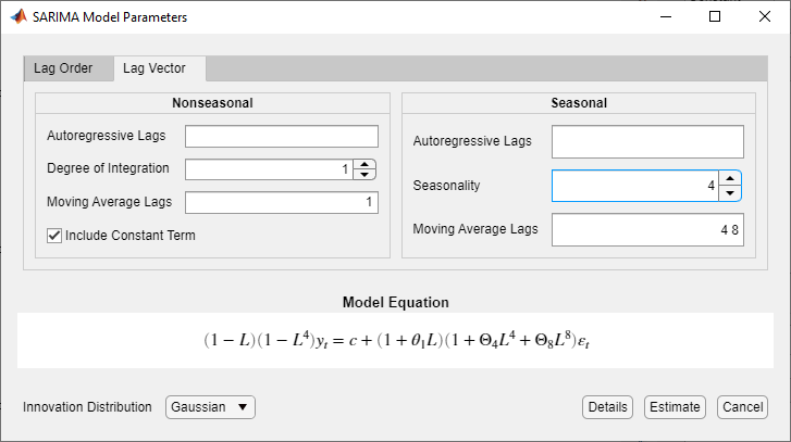
Specify Lag Structure Using Lag Vector Tab
On the Lag Vector tab, you specify the lags the lags that
comprise each seasonal and nonseasonal lag operator polynomial by typing a list of
nonnegative, unique integers in the corresponding box. Separate values by commas or
spaces, or use the colon operator (for example, 4:4:12). You
can specify at most two degrees of nonseasonal integration and one degree of
seasonal integration, and you can specify the data periodicity, by typing a
nonnegative integer in the appropriate box or by clicking
![]() .
.
Consider a SARIMA(0,1,1)×(0,1,2)4 model, a seasonal multiplicative ARIMA model with four periods in a season. To specify this model using the parameters in the Lag Vector tab:
Select a time series variable in the Time Series pane.
On the Modeler tab, in the Models section, click the arrow > SARIMA.
In the SARIMA Model Parameters dialog box, click the Lag Vector tab, then enter these values for the corresponding parameters.
In the Nonseasonal section, clear the Autoregressive Lags (p) box.
In the Seasonal section:
In the Seasonality box, type
4. A seasonal-difference polynomial of degree 4 appears in the equation.Clear the Autoregressive Lags (ps) box.
In the Moving Average Lags (qs) box, type
4 8. This action includes seasonal MA lags 4 and 8 in the equation.