Trend-Stationary vs. Difference-Stationary Processes
Nonstationary Processes
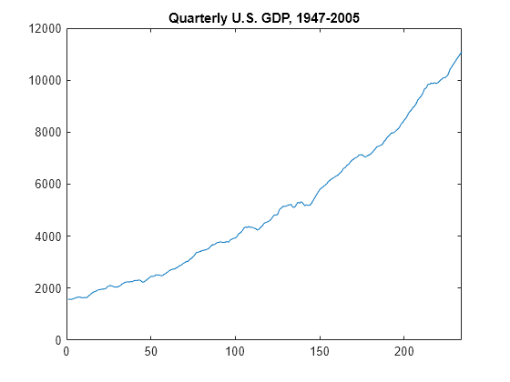
The stationary stochastic process is a building block of many econometric time series models. Many observed time series, however, have empirical features that are inconsistent with the assumptions of stationarity. For example, the following plot shows quarterly U.S. GDP measured from 1947 to 2005. There is a very obvious upward trend in this series that one should incorporate into any model for the process.
load Data_GDP
plot(Data)
xlim([0,234])
title('Quarterly U.S. GDP, 1947-2005')

A trending mean is a common violation of stationarity. There are two popular models for nonstationary series with a trending mean.
Trend stationary: The mean trend is deterministic. Once the trend is estimated and removed from the data, the residual series is a stationary stochastic process.
Difference stationary: The mean trend is stochastic. Differencing the series D times yields a stationary stochastic process.
The distinction between a deterministic and stochastic trend has important implications for the long-term behavior of a process:
Time series with a deterministic trend always revert to the trend in the long run (the effects of shocks are eventually eliminated). Forecast intervals have constant width.
Time series with a stochastic trend never recover from shocks to the system (the effects of shocks are permanent). Forecast intervals grow over time.
Unfortunately, for any finite amount of data there is a deterministic and stochastic trend that fits the data equally well (Hamilton, 1994). Unit root tests are a tool for assessing the presence of a stochastic trend in an observed series.
Trend Stationary
You can write a trend-stationary process, yt, as
where:
is a deterministic mean trend.
is a stationary stochastic process with mean zero.
In some applications, the trend is of primary interest. Time series decomposition methods focus on decomposing into different trend sources (e.g., secular trend component and seasonal component). You can decompose series nonparametrically using filters (moving averages), or parametrically using regression methods.
Given an estimate , you can explore the residual series for autocorrelation, and optionally model it using a stationary stochastic process model.
Difference Stationary
In the Box-Jenkins modeling approach [2], nonstationary time series are differenced until stationarity is achieved. You can write a difference-stationary process, yt, as
where:
is a Dth-degree differencing operator.
is an infinite-degree lag operator polynomial with absolutely summable coefficients and all roots lying outside the unit circle.
is an uncorrelated innovation process with mean zero.
Time series that can be made stationary by differencing are called integrated processes. Specifically, when D differences are required to make a series stationary, that series is said to be integrated of order D, denoted I(D). Processes with D ≥ 1 are often said to have a unit root.
References
[1] Hamilton, J. D. Time Series Analysis. Princeton, NJ: Princeton University Press, 1994.
[2] Box, G. E. P., G. M. Jenkins, and G. C. Reinsel. Time Series Analysis: Forecasting and Control. 3rd ed. Englewood Cliffs, NJ: Prentice Hall, 1994.