Using Bootstrapping and Filtered Historical Simulation to Evaluate Market Risk

Examine the Daily Closings of the Global Equity Index Data

The raw data consists of 2665 observations of daily closing values of the following representative equity indices spanning the trading dates 27-April-1993 to 14-July-2003:

  Canada: TSX Composite (Ticker ^GSPTSE)
  France: CAC 40        (Ticker ^FCHI)
 Germany: DAX           (Ticker ^GDAXI)
   Japan: Nikkei 225    (Ticker ^N225)
      UK: FTSE 100      (Ticker ^FTSE)
      US: S&P 500       (Ticker ^GSPC)

load Data_GlobalIdx1   % Import daily index closings
dt = datetime(dates,'ConvertFrom','datenum'); % Convert serial dates to datetimes

The following plot illustrates the relative price movements of each index. The initial level of each index has been normalized to unity to facilitate the comparison of relative performance, and no dividend adjustments are explicitly taken into account.

figure
plot(dt,ret2price(price2ret(Data)))
xlabel('Date')
ylabel('Index Value')
title ('Relative Daily Index Closings')
legend(series,Location='northwest')

In preparation for subsequent modeling, specify the portfolio weight vector. Although an equally weighted portfolio is assumed, you can change the weight vector to examine any other portfolio composition or even a single country. Note that the portfolio weights are fixed throughout the risk horizon, and that the simulation ignores any transaction costs required to rebalance the portfolio (the daily rebalancing process is assumed to be self-financing).

nIndices = size(Data,2);                    % # of indices
weights  = repmat(1/nIndices,nIndices,1);  % Equally weighted portfolio

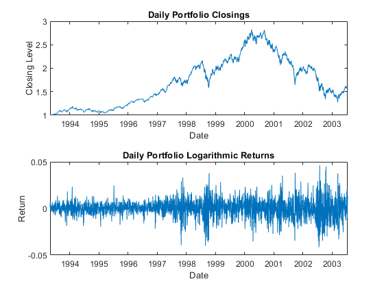
Given the weights, form the portfolio logarithmic return series (sometimes called geometric, or continuously compounded returns) from the daily returns of the individual indices. Although the index returns are logarithmic, the portfolio return series is constructed by first converting the individual logarithmic returns to arithmetic returns (price change divided by initial price), then weighting the individual arithmetic returns to obtain the arithmetic return of the portfolio, and finally converting back to portfolio logarithmic return. With daily data and a short VaR horizon, the repeated conversions make little difference, but for longer time periods the disparity may be significant.

returns = price2ret(Data,Method="periodic")*weights;    % Arithmetic returns
returns = log(1 + returns);                             % Logarithmic returns
T = size(returns,1);                                    % Historical sample size

Plot the daily closing value of the hypothetical portfolio along with the corresponding return series for comparison.

figure
tiledlayout(2,1)
nexttile
plot(dt,ret2price(returns))
xlabel('Date')
ylabel('Closing Level')
title('Daily Portfolio Closings')

nexttile
plot(dt(2:end),returns)
xlabel('Date')
ylabel('Return')
title('Daily Portfolio Logarithmic Returns')

Filter the Portfolio Returns

The bootstrapped FHS method requires the observations to be approximately independent and identically distributed. However, most financial return series exhibit some degree of autocorrelation and, more importantly, heteroskedasticity.

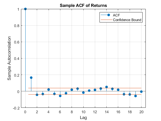
For example, the sample autocorrelation function (ACF) of the portfolio returns reveal some mild serial correlation.

figure
autocorr(returns)
title('Sample ACF of Returns')

However, the sample ACF of the squared returns illustrates the degree of persistence in variance and implies that GARCH modeling may significantly condition the data used in the subsequent bootstrapping method.

figure
autocorr(returns.^2)
title('Sample ACF of Squared Returns')

To produce a series of iid observations, fit a first order autoregressive model to the conditional mean of the portfolio returns

and an asymmetric exponential GARCH (EGARCH) model to the conditional variance

The first order autoregressive model compensates for autocorrelation, while the EGARCH model compensates for heteroskedasticity. In particular, the EGARCH model also incorporates asymmetry (leverage) into the variance equation (see [6]).

Additionally, the standardized residuals of each index are modeled as a standardized Student's t distribution to compensate for the fat tails often associated with equity returns. That is

iid distributed

The following code segment estimates the AR(1) + EGARCH(1,1) model and extracts the filtered residuals and conditional variances from the portfolio returns.

model = arima(AR=NaN,Distribution="t",Variance=egarch(1,1));
options = optimoptions(@fmincon,Display="off",Diagnostics="off", ...
    Algorithm="sqp",TolCon=1e-7);

fit = estimate(model,returns,Options=options);  % Fit the model
[residuals,variances] = infer(fit,returns);   % Infer residuals and variances

 
    ARIMA(1,0,0) Model (t Distribution):
 
                  Value       StandardError    TStatistic      PValue  
                __________    _____________    __________    __________

    Constant    0.00021376     0.00012471        1.7141        0.086507
    AR{1}          0.18549       0.019906        9.3186      1.1783e-20
    DoF             12.649         2.7038        4.6784      2.8914e-06

 
 
    EGARCH(1,1) Conditional Variance Model (t Distribution):
 
                     Value      StandardError    TStatistic      PValue  
                   _________    _____________    __________    __________

    Constant        -0.13366       0.030071       -4.4449       8.792e-06
    GARCH{1}         0.98639      0.0030907        319.15               0
    ARCH{1}          0.13383       0.019006        7.0417      1.8993e-12
    Leverage{1}    -0.091885       0.012152       -7.5616      3.9829e-14
    DoF               12.649         2.7038        4.6784      2.8914e-06

Compare the model residuals and the corresponding conditional standard deviations filtered from the raw returns. The lower graph clearly illustrates the variation in volatility (heteroskedasticity) present in the filtered residuals.

figure
tiledlayout(2,1)
nexttile
plot(dt(2:end), residuals)
xlabel('Date')
ylabel('Residual')
title ('Filtered Residuals')

nexttile
plot(dt(2:end), sqrt(variances))
xlabel('Date')
ylabel('Volatility')
title ('Filtered Conditional Standard Deviations')

Having filtered the model residuals from the portfolio return series, standardize each residual by the corresponding conditional standard deviation. These standardized residuals represent the underlying zero-mean, unit-variance, iid series. The iid property is important for bootstrapping, and allows the sampling procedure to safely avoid the pitfalls of sampling from a population in which successive observations are serially dependent.

standardizedResiduals = residuals./sqrt(variances);

To conclude this section, examine the ACFs of the standardized residuals and squared standardized residuals. Comparing the ACFs of the standardized residuals to the corresponding ACFs of the raw returns reveals that the standardized residuals are now approximately iid, thereby far more amenable to subsequent bootstrapping.

figure
autocorr(standardizedResiduals)
title('Sample ACF of Standardized Residuals')

figure
autocorr(standardizedResiduals.^2)
title('Sample ACF of Squared Standardized Residuals')

Simulate Global Index Portfolio Returns with FHS

As already mentioned, FHS bootstraps standardized residuals to generate paths of future asset returns and, therefore, makes no parametric assumptions about the probability distribution of those returns. The bootstrapping procedure produces iid standardized residuals consistent with those obtained from the AR(1) + EGARCH(1,1) filtering process above.

The following code segment simulates 20,000 independent random trials of standardized residuals over a one month horizon of 22 trading days.

s = RandStream.getGlobalStream();
reset(s)

nTrials = 20000;                  % # of independent random trials
horizon = 22;                     % VaR forecast horizon

bootstrappedResiduals = standardizedResiduals(unidrnd(T,horizon,nTrials));

Using the bootstrapped standardized residuals as the iid input noise process, reintroduce the autocorrelation and heteroskedasticity observed in the original portfolio return series via the Econometrics Toolbox™ filter function. To make the most of current information, specify the necessary presample model residuals, variances, and returns so that each simulated path evolves from a common initial state.

Y0 = returns(end);                            % Presample returns
Z0 = residuals(end)./sqrt(variances(end));    % Presample model standardized residuals
V0 = variances(end);                          % Presample variances

portfolioReturns = filter(fit,bootstrappedResiduals, ...
                         Y0=Y0,Z0=Z0,V0=V0);

Summarize the Results

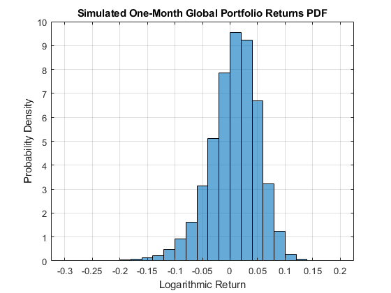
Having simulated the returns of the global index portfolio, report the maximum gain and loss, as well the VaR at various confidence levels, over the one month risk horizon. Also, plot the empirical cumulative distribution function (CDF) and the probability density function (PDF) of the portfolio cumulative returns.

Since you are working with daily logarithmic returns, the cumulative returns over the risk horizon are simply the sum of the returns over each intervening period.

cumulativeReturns = sum(portfolioReturns);

VaR = 100*quantile(cumulativeReturns,[0.10; 0.05; 0.01]);

disp(' ')
fprintf('Maximum Simulated Loss: %8.4f%s\n'   ,-100*min(cumulativeReturns),'%')
fprintf('Maximum Simulated Gain: %8.4f%s\n\n' ,100*max(cumulativeReturns),'%')
fprintf('     Simulated 90%% VaR: %8.4f%s\n'  ,VaR(1),'%')
fprintf('     Simulated 95%% VaR: %8.4f%s\n'  ,VaR(2),'%')
fprintf('     Simulated 99%% VaR: %8.4f%s\n\n',VaR(3),'%')

figure
h = cdfplot(cumulativeReturns);
h.Color = 'Red';
xlabel('Logarithmic Return')
ylabel('Probability')
title ('Simulated One-Month Global Portfolio Returns CDF')

figure
bins = -0.3:0.02:0.2;
histogram(cumulativeReturns,bins,Normalization="pdf")
xlabel('Logarithmic Return')
ylabel('Probability Density')
title ('Simulated One-Month Global Portfolio Returns PDF')
grid on

 
Maximum Simulated Loss:  39.7595%
Maximum Simulated Gain:  15.2458%

     Simulated 90% VaR:  -5.0145%
     Simulated 95% VaR:  -7.2182%
     Simulated 99% VaR: -12.4881%

References

[1] Barone-Adesi, G., K. Giannopoulos, and L. Vosper. "VaR without Correlations for Non-Linear Portfolios." Journal of Futures Markets. Vol. 19, 1999, pp. 583–602.
[2] Brandolini, D., M. Pallotta, and R. Zenti. "Risk Management in an Asset Management Company: A Practical Case." Presented at EMFA 2001, Lugano, Switzerland. 2000.
[3] Christoffersen, P.F. Elements of Financial Risk Management. Waltham, MA: Academic Press, 2002.
[4] Dowd, K. Measuring Market Risk. West Sussex: John Wiley & Sons, 2005.
[5] McNeil, A. and R. Frey. "Estimation of Tail Related Risk Measure for Heteroscedastic Financial Time Series: An Extreme Value Approach." Journal of Empirical Finance. Vol. 7, 2000, pp. 271–300.
[6] Nelson, D. B. "Conditional Heteroskedasticity in Asset Returns: A New Approach." Econometrica.. Vol. 59, No. 2, 1991, pp. 347–370.