lifetableconv
Convert life table series into life tables with forced termination
Description
Examples
Load the life table data file.
load us_lifetable_2009Convert life table series into life tables with forced termination.
[qx,lx,dx] = lifetableconv(x,lx);
display(qx(1:20,:))
    0.0064    0.0070    0.0057
    0.0004    0.0004    0.0004
    0.0003    0.0003    0.0002
    0.0002    0.0002    0.0002
    0.0002    0.0002    0.0001
    0.0001    0.0002    0.0001
    0.0001    0.0001    0.0001
    0.0001    0.0001    0.0001
    0.0001    0.0001    0.0001
    0.0001    0.0001    0.0001
    0.0001    0.0001    0.0001
    0.0001    0.0001    0.0001
    0.0001    0.0001    0.0001
    0.0002    0.0002    0.0002
    0.0003    0.0004    0.0002
    0.0004    0.0005    0.0002
    0.0005    0.0006    0.0003
    0.0005    0.0007    0.0003
    0.0006    0.0009    0.0004
    0.0007    0.0010    0.0004
display(lx(1:20,:))
   1.0e+05 *

    1.0000    1.0000    1.0000
    0.9936    0.9930    0.9943
    0.9932    0.9926    0.9939
    0.9930    0.9923    0.9937
    0.9927    0.9920    0.9935
    0.9926    0.9919    0.9933
    0.9924    0.9917    0.9932
    0.9923    0.9916    0.9931
    0.9922    0.9914    0.9930
    0.9921    0.9913    0.9929
    0.9920    0.9912    0.9928
    0.9919    0.9911    0.9927
    0.9918    0.9910    0.9926
    0.9917    0.9909    0.9925
    0.9915    0.9907    0.9923
    0.9912    0.9903    0.9921
    0.9908    0.9898    0.9919
    0.9904    0.9892    0.9916
    0.9899    0.9885    0.9913
    0.9892    0.9876    0.9909
display(dx(1:20,:))
  637.2266  698.8750  572.6328
   40.4062   43.9297   36.7188
   27.1875   30.0938   24.1406
   20.7656   23.0781   18.3359
   15.9141   17.2109   14.5625
   14.8672   16.3125   13.3516
   13.3672   14.7891   11.8750
   12.1328   13.3828   10.8203
   10.8125   11.6094    9.9844
    9.4609    9.5781    9.3438
    8.6172    8.1328    9.1172
    9.2656    8.8359    9.7188
   12.5938   13.5078   11.6328
   19.1016   22.9844   15.0234
   27.6719   35.5938   19.3516
   36.6328   48.5703   24.0547
   45.0156   60.7109   28.4844
   53.1406   72.8906   32.2812
   60.8984   85.1172   35.2578
   68.3438   97.2266   37.6875
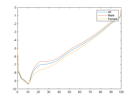
Plot the qx series and display the legend. The series qx is the conditional probability that a person at age x will die between age x and the next age in the series.
plot(x,log(qx))
legend(series)
Load the life table data file.
load us_lifetable_2009Calibrate life table from survival data with the default Heligman-Pollard parametric model.
a = lifetablefit(x,lx)
a = 8×3

    0.0005    0.0006    0.0004
    0.0592    0.0819    0.0192
    0.1452    0.1626    0.1048
    0.0007    0.0011    0.0007
    6.2846    6.7639    1.1037
   24.1388   24.2895   53.1830
    0.0000    0.0000    0.0000
    1.0971    1.0987    1.1100
Generate life table series from the calibrated mortality model.
qx = lifetablegen((0:120),a);
display(qx(1:20,:))
    0.0063    0.0069    0.0057
    0.0005    0.0006    0.0004
    0.0002    0.0003    0.0002
    0.0002    0.0002    0.0002
    0.0001    0.0001    0.0001
    0.0001    0.0001    0.0001
    0.0001    0.0001    0.0001
    0.0001    0.0001    0.0001
    0.0001    0.0001    0.0001
    0.0001    0.0001    0.0001
    0.0001    0.0001    0.0001
    0.0001    0.0001    0.0001
    0.0002    0.0002    0.0001
    0.0002    0.0002    0.0002
    0.0002    0.0003    0.0002
    0.0003    0.0004    0.0002
    0.0004    0.0005    0.0002
    0.0005    0.0006    0.0003
    0.0006    0.0008    0.0003
    0.0007    0.0009    0.0003
Convert life table series into life tables with forced termination.
[~,~,dx] = lifetableconv((0:120),qx,'qx');
display(dx(1:20,:))
630.9947 686.9478 571.6096 48.7922 55.1033 40.9864 24.8017 26.3779 23.6166 17.0832 17.5878 17.0318 13.6183 13.8188 13.6144 11.8663 12.0076 11.6316 10.9783 11.1573 10.4906 10.5997 10.8604 9.9489 10.5759 10.9396 9.8953 10.8790 11.3612 10.2718 11.6084 12.2508 11.0418 12.9919 13.9271 12.1762 15.3474 16.8834 13.6480 18.9930 21.6791 15.4298 24.1381 28.7662 17.4940 30.7992 38.3211 19.8130 38.7701 50.1486 22.3600 47.6521 63.6906 25.1094 56.9291 78.1269 28.0382 66.0571 92.5259 31.1254
Plot the dx series and display the legend. The series dx is the number of people who die out of 100,000 alive at birth between age x and the next age in the series.
plot((0:119),dx(1:end-1,:));
legend(series, 'location', 'northwest');
title('\bfLife Table Yearly Decrements');
xlabel('Age');
ylabel('Number Dying within a Given Year');

Input Arguments
Output Arguments
More About
Most modern life tables have “forced” termination. Forced termination means that the last row of the life table applies for all persons with ages on or after the last age in the life table.
This sample illustrates forced termination.
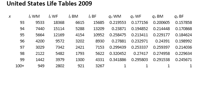
In this case, the last row of the life table applies for all persons aged 100 or older. Specifically, qx probabilities are 1qx for ages less than 100 and, technically, ∞qx for age 100.
Forced termination has terminal age values that apply to all ages after the
terminal age so that lx is positive, qx is
1, and dx is positive. Ages after the
terminal age are NaN values, although lx and
dx can be 0 and qx can
be 1 for input series. Forced termination is triggered by a
naturally terminating series, the last age in a truncated series, or the first
NaN value in a series.
Before 1970, life tables were often published with data that included all ages for which persons associated with a given series were still alive. Tables in this form have "natural" termination. In natural termination, the last row of the life table for each series counts the deaths or probabilities of deaths of the last remaining person at the corresponding age. Tables in this form can be problematic due to the granularity of the data and the fact that groups of series can terminate at distinct ages. Natural termination is illustrated in the following sample of the last few years of a life table.
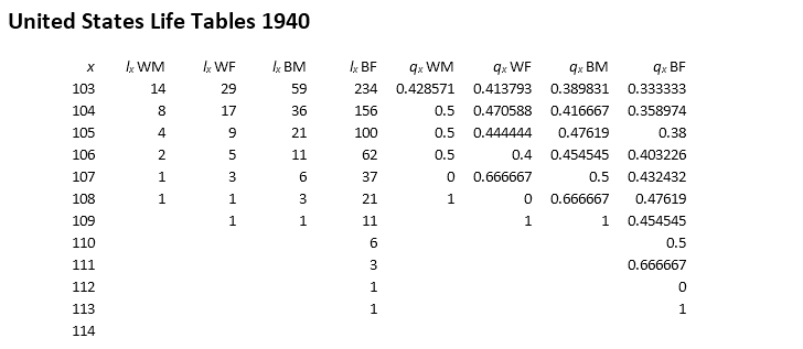
This form for life tables poses a number of issues that go beyond the obvious
statistical issues. First, the
lx table on the
left terminates at ages 108, 109, 109, and 113 for the four series in the table.
Technically, the numbers after these ages are 0, but can also be
NaN values because no person is alive after these terminating
ages. Second, the probabilities
qx on the right
terminate with fluctuating probabilities that go from 0 to
1 in some cases. In this case, however, all probabilities are
1qx
probabilities (unlike the forced termination probabilities). You can argue that the
probabilities after the ages of termination can be 1 (anyone
alive at this age is expected to die in the next year), 0 (the
age lies outside the support of the probability distribution), or
NaN values.
Truncated termination occurs with truncation of life tables at an
arbitrary age. For example, from 1970–1990, United States life tables truncated at
age 85. This format is problematic because life table probabilities must either
terminate with probability 1 (forced termination) or discard data
that exceeds the terminating age. This sample of the last few years of a life table
illustrates truncated termination. The raw data for this table is the
lx series. The
qx series is
derived from this series.
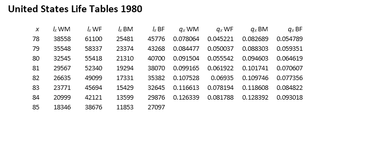
This life table format poses problems for termination because, for example, over 27% of the population for the fourth lx series is still alive at age 85. To claim that the probability of dying for all ages after age 85 is 100% might be true but is uninformative. Notwithstanding the statistical issues, however, tables in this form are completed by forced termination.
References
[1] Arias, E. “United States Life Tables.” National Vital Statistics Reports, U.S. Department of Health and Human Services. Vol. 62, No. 7, 2009.
Version History
Introduced in R2015a