Fitting the Diebold Li Model

Open Live Script

This example shows how to construct a Diebold Li model of the US yield curve for each month from 1990 to 2010. This example also demonstrates how to forecast future yield curves by fitting an autoregressive model to the time series of each parameter.

This example is based on the following paper:

https://www.nber.org/papers/w10048

Load the Data

The data used are monthly Treasury yields from 1990 through 2010 for tenors of 1 Mo, 3 Mo, 6 Mo, 1 Yr, 2 Yr, 3 Yr, 5 Yr, 7 Yr, 10 Yr, 20 Yr, 30 Yr.

Daily data can be found here:

https://www.treasury.gov/resource-center/data-chart-center/interest-rates/Pages/TextView.aspx?data=yieldAll

Data is stored in a MATLAB® data file as a timetable.

opts = detectImportOptions("dailyYieldData.xlsx");
opts = setvartype(opts,"double");
opts = setvartype(opts,"Time","datetime");
dailyData = readtimetable("dailyYieldData.xlsx", opts)

dailyData=5256×11 timetable
       Time        x1M     x3M       x6M       x1Y       x2Y       x3Y       x5Y       x7Y       x10Y     x20Y     x30Y 
    ___________    ___    ______    ______    ______    ______    ______    ______    ______    ______    ____    ______

    02-Jan-1990    NaN    0.0783    0.0789    0.0781    0.0787     0.079    0.0787    0.0798    0.0794    NaN       0.08
    03-Jan-1990    NaN    0.0789    0.0794    0.0785    0.0794    0.0796    0.0792    0.0804    0.0799    NaN     0.0804
    04-Jan-1990    NaN    0.0784     0.079    0.0782    0.0792    0.0793    0.0791    0.0802    0.0798    NaN     0.0804
    05-Jan-1990    NaN    0.0779    0.0785    0.0779     0.079    0.0794    0.0792    0.0803    0.0799    NaN     0.0806
    08-Jan-1990    NaN    0.0779    0.0788    0.0781     0.079    0.0795    0.0792    0.0805    0.0802    NaN     0.0809
    09-Jan-1990    NaN     0.078    0.0782    0.0778    0.0791    0.0794    0.0792    0.0805    0.0802    NaN      0.081
    10-Jan-1990    NaN    0.0775    0.0778    0.0777    0.0791    0.0795    0.0792      0.08    0.0803    NaN     0.0811
    11-Jan-1990    NaN     0.078     0.078    0.0777    0.0791    0.0795    0.0794    0.0801    0.0804    NaN     0.0811
    12-Jan-1990    NaN    0.0774    0.0781    0.0776    0.0793    0.0798    0.0799    0.0807     0.081    NaN     0.0817
    16-Jan-1990    NaN    0.0789    0.0799    0.0792     0.081    0.0813    0.0811    0.0818     0.082    NaN     0.0825
    17-Jan-1990    NaN    0.0797    0.0797    0.0791    0.0809    0.0811    0.0811    0.0817    0.0819    NaN     0.0825
    18-Jan-1990    NaN    0.0804    0.0808    0.0805    0.0825    0.0828    0.0827    0.0831    0.0832    NaN     0.0835
    19-Jan-1990    NaN      0.08    0.0801      0.08     0.082    0.0823     0.082    0.0824    0.0826    NaN     0.0829
    22-Jan-1990    NaN    0.0799    0.0799    0.0798    0.0818     0.082    0.0819    0.0825    0.0827    NaN     0.0831
    23-Jan-1990    NaN    0.0793    0.0797    0.0797    0.0818     0.082    0.0818    0.0823    0.0826    NaN     0.0829
    24-Jan-1990    NaN    0.0793    0.0799      0.08     0.082    0.0829    0.0828    0.0834    0.0838    NaN     0.0841
      ⋮

Extract data for the last day of each month.

Estimationdataset = retime(dailyData, "monthly", "lastvalue")

Estimationdataset=252×11 timetable
       Time        x1M     x3M       x6M       x1Y       x2Y       x3Y       x5Y       x7Y       x10Y     x20Y     x30Y 
    ___________    ___    ______    ______    ______    ______    ______    ______    ______    ______    ____    ______

    01-Jan-1990    NaN      0.08    0.0813    0.0808    0.0828    0.0836    0.0835    0.0839    0.0843    NaN     0.0846
    01-Feb-1990    NaN    0.0804    0.0814    0.0812    0.0843    0.0845    0.0844    0.0854    0.0851    NaN     0.0854
    01-Mar-1990    NaN    0.0807    0.0824    0.0835    0.0864    0.0869    0.0865     0.087    0.0865    NaN     0.0863
    01-Apr-1990    NaN    0.0807    0.0844    0.0858    0.0896    0.0905    0.0904    0.0906    0.0904    NaN       0.09
    01-May-1990    NaN    0.0801    0.0812    0.0822     0.085    0.0853    0.0856    0.0864     0.086    NaN     0.0858
    01-Jun-1990    NaN      0.08    0.0802    0.0805    0.0824    0.0832    0.0835    0.0846    0.0843    NaN     0.0841
    01-Jul-1990    NaN    0.0774    0.0772    0.0772    0.0791    0.0804    0.0813    0.0828    0.0836    NaN     0.0842
    01-Aug-1990    NaN    0.0763    0.0774    0.0776    0.0807    0.0826     0.085    0.0877    0.0886    NaN     0.0899
    01-Sep-1990    NaN    0.0737    0.0754    0.0769    0.0802    0.0819    0.0847    0.0873    0.0882    NaN     0.0896
    01-Oct-1990    NaN    0.0734    0.0746    0.0743    0.0777    0.0797    0.0824     0.085    0.0865    NaN     0.0878
    01-Nov-1990    NaN    0.0724    0.0736    0.0731    0.0753    0.0767    0.0791    0.0818    0.0826    NaN      0.084
    01-Dec-1990    NaN    0.0663    0.0673    0.0682    0.0715     0.074    0.0768      0.08    0.0808    NaN     0.0826
    01-Jan-1991    NaN    0.0637    0.0649    0.0651    0.0705     0.073    0.0762    0.0789    0.0803    NaN     0.0821
    01-Feb-1991    NaN    0.0622    0.0632    0.0641    0.0704    0.0726    0.0766    0.0789    0.0802    NaN     0.0819
    01-Mar-1991    NaN    0.0592    0.0605    0.0628    0.0702     0.073    0.0773    0.0796    0.0805    NaN     0.0824
    01-Apr-1991    NaN    0.0568    0.0583    0.0606     0.068    0.0715    0.0763    0.0788    0.0802    NaN      0.082
      ⋮

EstimationData = table2array(Estimationdataset)

EstimationData = 252×11

       NaN    0.0800    0.0813    0.0808    0.0828    0.0836    0.0835    0.0839    0.0843       NaN    0.0846
       NaN    0.0804    0.0814    0.0812    0.0843    0.0845    0.0844    0.0854    0.0851       NaN    0.0854
       NaN    0.0807    0.0824    0.0835    0.0864    0.0869    0.0865    0.0870    0.0865       NaN    0.0863
       NaN    0.0807    0.0844    0.0858    0.0896    0.0905    0.0904    0.0906    0.0904       NaN    0.0900
       NaN    0.0801    0.0812    0.0822    0.0850    0.0853    0.0856    0.0864    0.0860       NaN    0.0858
       NaN    0.0800    0.0802    0.0805    0.0824    0.0832    0.0835    0.0846    0.0843       NaN    0.0841
       NaN    0.0774    0.0772    0.0772    0.0791    0.0804    0.0813    0.0828    0.0836       NaN    0.0842
       NaN    0.0763    0.0774    0.0776    0.0807    0.0826    0.0850    0.0877    0.0886       NaN    0.0899
       NaN    0.0737    0.0754    0.0769    0.0802    0.0819    0.0847    0.0873    0.0882       NaN    0.0896
       NaN    0.0734    0.0746    0.0743    0.0777    0.0797    0.0824    0.0850    0.0865       NaN    0.0878
      ⋮

dates = Estimationdataset.Properties.RowTimes;

Diebold Li Model

Diebold and Li start with the Nelson Siegel model

$y = β_{0} + (β_{1} + β_{2}) \frac{τ}{m} (1 - e^{\frac{- m}{τ}}) - β_{2} e^{\frac{- m}{τ}}$

and rewrite it to be the following:

$y_{t} (τ) = β_{1 t} + β_{2 t} (\frac{1 - e^{- λ_{t} τ}}{λ_{t} τ}) + β_{3 t} (\frac{1 - e^{- λ_{t} τ}}{λ_{t} τ} - e^{- λ_{t} τ})$

The above model allows the factors to be interpreted in the following way: Beta1 corresponds to the long term/level of the yield curve, Beta2 corresponds to the short term/slope, and Beta3 corresponds to the medium term/curvature. $λ$ determines the maturity at which the loading on the curvature is maximized, and governs the exponential decay rate of the model.

Diebold and Li advocate setting $λ$ to maximize the loading on the medium term factor, Beta3, at 30 months. This also transforms the problem from a nonlinear fitting to a simple linear regression.

% Explicitly set the time factor lambda
lambda_t = .0609;

% Construct a matrix of the factor loadings
% Tenors associated with data
TimeToMat = [3 6 9 12 24 36 60 84 120 240 360]';
X = [ones(size(TimeToMat)) (1 - exp(-lambda_t*TimeToMat))./(lambda_t*TimeToMat) ...
    ((1 - exp(-lambda_t*TimeToMat))./(lambda_t*TimeToMat) - exp(-lambda_t*TimeToMat))];

% Plot the factor loadings
plot(TimeToMat,X)
title("Factor Loadings for Diebold Li Model with time factor of .0609")
xlabel("Maturity (months)")
ylim([0 1.1])
legend(["Beta1","Beta2","Beta3"],"location","east")

Figure contains an axes object. The axes object with title Factor Loadings for Diebold Li Model with time factor of .0609, xlabel Maturity (months) contains 3 objects of type line. These objects represent Beta1, Beta2, Beta3.

Fit the Model

A DieboldLi object is developed to facilitate fitting the model from yield data. The DieboldLi object inherits from the IRCurve object, so the getZeroRates, getDiscountFactors, getParYields, getForwardRates, and toRateSpec methods are all implemented. Additionally, the method fitYieldsFromBetas is implemented to estimate the Beta parameters given a lambda parameter for observed market yields.

The DieboldLi object is used to fit a Diebold Li model for each month from 1990 through 2010.

% Preallocate the Betas
Beta = zeros(size(EstimationData,1),3);

% Loop through and fit each end of month yield curve
for jdx = 1:size(EstimationData,1)
    tmpCurveModel = DieboldLi.fitBetasFromYields(dates(jdx),lambda_t*12,dates(jdx) + calmonths(TimeToMat),EstimationData(jdx,:)');
    Beta(jdx,:) = [tmpCurveModel.Beta1 tmpCurveModel.Beta2 tmpCurveModel.Beta3];
end

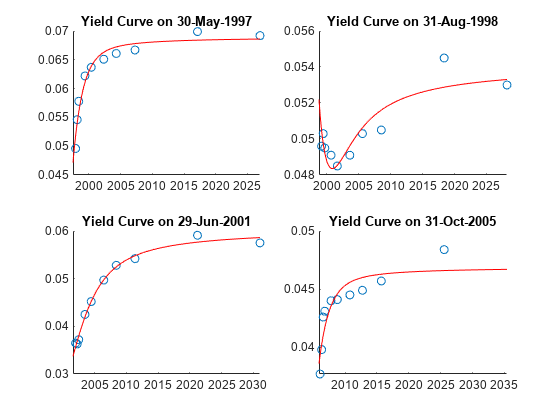
The Diebold Li fits on selected dates are included here. While this example uses EOM data, the time stamps are for the first of each month.

PlotSettles = datetime([1997, 1998, 2001, 2005], [5,8,6,10], 1);

lambda_annual = lambda_t*12;
for jdx = 1:length(PlotSettles)
    subplot(2,2,jdx)
    tmpIdx = find(PlotSettles(jdx)==dates);
    tmpCurveModel = DieboldLi.fitBetasFromYields(PlotSettles(jdx),lambda_annual,...
        PlotSettles(jdx)+calmonths(TimeToMat),EstimationData(tmpIdx,:)');
    scatter(PlotSettles(jdx)+calmonths(TimeToMat),EstimationData(tmpIdx,:))
    hold on
    PlottingDates = PlotSettles(jdx)+calmonths(1:360)';
    plot(PlottingDates,tmpCurveModel.getParYields(PlottingDates),"r-")
    hold off
    title("Yield Curve on " + datestr(dateshift(PlotSettles(jdx), "end", "month")))
end

Forecasting

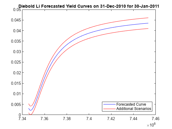
The Diebold Li model can be used to forecast future yield curves. Diebold and Li propose fitting an AR(1) model to the time series of each Beta parameter. This fitted model is then used to forecast future values of each parameter, and by extension, future yield curves.

For this example the MATLAB function fitlm is used to estimate the parameters for an AR(1) model for each Beta.

The confidence intervals for the regression fit are also used to generate two additional yield curve forecasts that serve as additional possible scenarios for the yield curve.

You can adjust The MonthsLag variable to make different period ahead forecasts. For example, changing the value from 1 to 6 would change the forecast from a 1 month ahead to a 6 months ahead forecast.

MonthsLag = 1;

ForecastBeta = zeros(1,3);
ForecastBeta_Down = zeros(1,3);
ForecastBeta_Up = zeros(1,3);

for k = 1:3 % for each Beta
    currentFit = fitlm( Beta(1:end-MonthsLag,k), Beta(MonthsLag+1:end,k));
    tmpBeta = currentFit.Coefficients.Estimate;
    bint = coefCI(currentFit);
    
    ForecastBeta(k) = [1 Beta(end,k)]*tmpBeta;
    ForecastBeta_Down(k) = [1 Beta(end,k)]*bint(:,1);
    ForecastBeta_Up(k) = [1 Beta(end,k)]*bint(:,2);
end

% Forecasted yield curve
figure
Settle = dates(end) + calmonths(MonthsLag);
DieboldLi_Forecast = DieboldLi("ParYield",Settle,[ForecastBeta lambda_annual]);
DieboldLi_Forecast_Up = DieboldLi("ParYield",Settle,[ForecastBeta_Up lambda_annual]);
DieboldLi_Forecast_Down = DieboldLi("ParYield",Settle,[ForecastBeta_Down lambda_annual]);
PlottingDates = Settle+calmonths(1:360)';
plot(PlottingDates,DieboldLi_Forecast.getParYields(PlottingDates),"b-")
hold on
plot(PlottingDates,DieboldLi_Forecast_Up.getParYields(PlottingDates),"r-")
plot(PlottingDates,DieboldLi_Forecast_Down.getParYields(PlottingDates),"r-")
hold off
title("Diebold Li Forecasted Yield Curves on " + datestr(dates(end)) + " for " + datestr(Settle))
legend(["Forecasted Curve","Additional Scenarios"],"location","southeast")

Figure contains an axes object. The axes object with title Diebold Li Forecasted Yield Curves on 01-Dec-2010 for 01-Jan-2011 contains 3 objects of type line. These objects represent Forecasted Curve, Additional Scenarios.

Bibliography

This example is based on the following paper:

[1] Francis X. Diebold, Canlin Li. "Forecasting the Term Structure of Government Bond Yields." Journal of Econometrics, Volume 130, Issue 2, February 2006, pp. 337–364.