Hedging Functions
Introduction
Hedging is an investment to reduce the risk of adverse price movements in an asset.
Financial Instruments Toolbox™ offers two functions for assessing the fundamental hedging tradeoff, hedgeopt and hedgeslf.
The first function, hedgeopt, addresses the most general
hedging problem. It allocates an optimal hedge to satisfy either of two goals:
Minimize the cost of hedging a portfolio given a set of target sensitivities.
Minimize portfolio sensitivities for a given set of maximum target costs.
hedgeopt allows investors
to modify portfolio allocations among instruments according to either
of the goals. The problem is cast as a constrained linear least-squares
problem. For additional information about hedgeopt,
see Hedging with hedgeopt.
The second function, hedgeslf, attempts to allocate a
self-financing hedge among a portfolio of instruments. In particular, hedgeslf attempts to maintain a constant portfolio value consistent with
reduced portfolio sensitivities (that is, the rebalanced portfolio is hedged against market
moves and is closest to being self-financing). If hedgeslf cannot find a self-financing hedge, it rebalances the portfolio to
minimize overall portfolio sensitivities. For additional information on hedgeslf, see Self-Financing Hedges with hedgeslf.
The examples in this section consider the delta,
gamma, and vega sensitivity measures. In this
toolbox, when you work with interest-rate derivatives, delta is the
price sensitivity measure of shifts in the forward yield curve, gamma is the delta
sensitivity measure of shifts in the forward yield curve, and vega is the price sensitivity
measure of shifts in the volatility process. See bdtsens or hjmsens for details on the computation of
sensitivities for interest-rate derivatives.
For equity exotic options, the underlying
instrument is the stock price instead of the forward yield curve.
So, delta now represents the price sensitivity measure of shifts in
the stock price, gamma is the delta sensitivity measure of shifts
in the stock price, and vega is the price sensitivity measure of shifts
in the volatility of the stock. See crrsens, eqpsens, ittsens,
or sttsens for details on the
computation of sensitivities for equity derivatives.
For examples showing the computation of sensitivities for interest-rate based derivatives, see Computing Instrument Sensitivities. Likewise, for examples showing the computation of sensitivities for equity exotic options, see Computing Equity Instrument Sensitivities.
Note
The delta, gamma, and vega sensitivities that the toolbox calculates are dollar sensitivities.
Hedging with hedgeopt
This example shows hedging options for a portfolio when using hedgeopt. To illustrate the hedging facility, consider the portfolio HWInstSet obtained from the file deriv.mat. The portfolio consists of eight instruments: two bonds, one bond option, one fixed-rate note, one floating-rate note, one cap, one floor, and one swap.
Load the example portfolio and use hwsens to compute the price and sensitivities.
load deriv.mat
format bank
[Delta, Gamma, Vega, Price] = hwsens(HWTree, HWInstSet);
Extract the current portfolio holdings.
Holdings = instget(HWInstSet, 'FieldName', 'Quantity');
For convenience place the delta, gamma, and vega sensitivity measures into a matrix of sensitivities.
Sensitivities = [Delta Gamma Vega];
Each row of the Sensitivities matrix is associated with a different instrument in the portfolio, and each column with a different sensitivity measure.
To summarize the portfolio information:
disp([Price Holdings Sensitivities])
        100.92         20.00       -291.26        858.41             0
         99.33         15.00       -374.64       1460.88         -0.00
          4.80        -10.00       -200.84      26835.26        119.40
        102.99         25.00       -383.57       1487.24         -0.00
        100.28          5.00         -0.55          1.28          0.00
          0.58         10.00         60.96       5599.37        113.38
          2.10          5.00       -209.24       8205.31        122.88
          8.78          8.00       -306.78        894.26         -0.00
The first column above is the dollar unit price of each instrument, the second is the holdings of each instrument (the quantity held or the number of contracts), and the third, fourth, and fifth columns are the dollar delta, gamma, and vega sensitivities, respectively.
The current portfolio sensitivities are a weighted average of the instruments in the portfolio.
TargetSens = Holdings' * Sensitivities
TargetSens = 1×3

     -21919.18     -87909.38        554.13
Maintaining Existing Allocations
Using hedgeopt, suppose that you want to maintain your existing portfolio. The first form of hedgeopt minimizes the cost of hedging a portfolio given a set of target sensitivities. If you want to maintain your existing portfolio composition and exposure, you should be able to do so without spending any money. To verify this, set the target sensitivities to the current sensitivities.
FixedInd = [1 2 3 4 5 6 7 8];
[Sens, Cost, Quantity] = hedgeopt(Sensitivities, Price,Holdings, FixedInd, [], [], TargetSens)
Sens = 1×3

     -21919.18     -87909.38        554.13
Cost =
             0
Quantity = 1×8

         20.00         15.00        -10.00         25.00          5.00         10.00          5.00          8.00
Portfolio composition and sensitivities are unchanged, and the cost associated with doing nothing is zero. The cost is defined as the change in portfolio value. This number cannot be less than zero because the rebalancing cost is defined as a nonnegative number.
If Value0 and Value1 represent the portfolio value before and after rebalancing, respectively, the zero cost can also be verified by comparing the portfolio values.
Value0 = Holdings' * Price
Value0 =
       6623.00
Partially Hedged Portfolio
Suppose you want to know the cost to achieve an overall portfolio dollar sensitivity of [-23000 -3300 3000], while allowing trading only in instruments 2, 3, and 6 (holding the positions of instruments 1, 4, 5, 7, and 8 fixed). To find the cost, first set the target portfolio dollar sensitivity.
TargetSens = [-23000 -3300 3000];
Specify the instruments to be fixed.
FixedInd = [1 4 5 7 8];
Then use hedgeopt.
[Sens, Cost, Quantity] = hedgeopt(Sensitivities, Price, ...
Holdings, FixedInd, [], [], TargetSens);
Recompute Value1, the portfolio value after rebalancing.
Value1 = Quantity * Price
Value1 =
       7421.98
Fully Hedged Portfolio
You can compute the cost associated with a fully hedged portfolio (simultaneous delta, gamma, and vega neutrality). In this case, set the target sensitivity to a row vector of 0s and use hedgeopt.
TargetSens = [0 0 0];
[Sens, Cost, Quantity] = hedgeopt(Sensitivities, Price, ...
Holdings, FixedInd, [], [], TargetSens);
Calculate the new portfolio value.
Value1 = Quantity * Price
Value1 =
         59.23
Minimizing Portfolio Sensitivities
You can use hedgeopt to determine the minimum cost of hedging a portfolio given a set of target sensitivities. In the following code, portfolio target sensitivities are treated as equality constraints during the optimization process. You tell hedgeopt what sensitivities you want, and it tells you what it will cost to get those sensitivities.
A related problem involves minimizing portfolio sensitivities for a given set of maximum target costs. For this goal, the target costs are treated as inequality constraints during the optimization process. You tell hedgeopt the most you are willing spend to insulate your portfolio, and it tells you the smallest portfolio sensitivities you can get for your money.
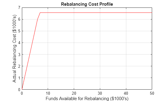
To illustrate this use of hedgeopt, compute the portfolio dollar sensitivities along the entire cost frontier. Assume, for example, you are willing to spend as much as $50,000, and want to see what portfolio sensitivities will result along the cost frontier. Assume that the same instruments are held fixed, and that the cost frontier is evaluated from $0 to $50,000 at increments of $1000.
MaxCost = [0:1000:50000];
[Sens, Cost, Quantity] = hedgeopt(Sensitivities, Price, ...
Holdings, FixedInd, [], MaxCost);
With this data, you can plot the required hedging cost versus the funds available (the amount you are willing to spend).
plot(MaxCost/1000, Cost/1000, 'red'), grid
xlabel('Funds Available for Rebalancing ($1000''s)')
ylabel('Actual Rebalancing Cost ($1000''s)')
title ('Rebalancing Cost Profile')
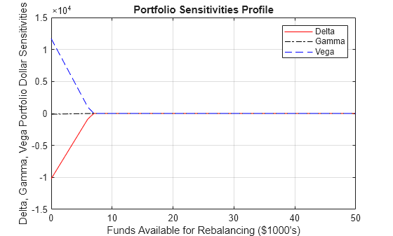
Also, you can plot the portfolio dollar sensitivities versus the funds available.
figure
plot(MaxCost/1000, Sens(:,1), '-red')
hold('on')
plot(MaxCost/1000, Sens(:,2), '-.black')
plot(MaxCost/1000, Sens(:,3), '--blue')
grid
xlabel('Funds Available for Rebalancing ($1000''s)')
ylabel('Delta, Gamma, Vega Portfolio Dollar Sensitivities')
title ('Portfolio Sensitivities Profile')
legend('Delta', 'Gamma', 'Vega')
Self-Financing Hedges with hedgeslf
This example shows how to find the point of delta, gamma, and vega neutrality using hedgeslf.
Load the example portfolio and use hwsens to compute the price and sensitivities.
load deriv.mat
format bank
[Delta, Gamma, Vega, Price] = hwsens(HWTree, HWInstSet);
Extract the current portfolio holdings.
Holdings = instget(HWInstSet, 'FieldName', 'Quantity');
For convenience place the delta, gamma, and vega sensitivity measures into a matrix of sensitivities.
Sensitivities = [Delta Gamma Vega];
Each row of the Sensitivities matrix is associated with a different instrument in the portfolio, and each column with a different sensitivity measure.
To summarize the portfolio information:
disp([Price Holdings Sensitivities])
        100.92         20.00       -291.26        858.41             0
         99.33         15.00       -374.64       1460.88         -0.00
          4.80        -10.00       -200.84      26835.26        119.40
        102.99         25.00       -383.57       1487.24         -0.00
        100.28          5.00         -0.55          1.28          0.00
          0.58         10.00         60.96       5599.37        113.38
          2.10          5.00       -209.24       8205.31        122.88
          8.78          8.00       -306.78        894.26         -0.00
Find the point of delta, gamma, and vega neutrality using hedgeslf.
FixedInd = [1 2 3 5 7 8];
[Sens, Value1, Quantity] = hedgeslf(Sensitivities, Price, ...
Holdings, FixedInd)
Sens = 3×1

    -205354.69
   -8763957.63
    -181824.04
Value1 =
      28607.83
Quantity = 8×1

         20.00
         15.00
        -10.00
        247.59
          5.00
      -1598.59
          5.00
          8.00
Similar to hedgeopt, hedgeslf returns the portfolio dollar sensitivities and instrument quantities (the rebalanced holdings). hedgeslf finds the best possible solution required to obtain zero sensitivities.
There is a syntax available for hedgeopt directly related to the results for hedgeslf. Suppose, instead of directly specifying the funds available for rebalancing (the most money you are willing to spend), you want to simply specify the number of points along the cost frontier. This call to hedgeopt samples the cost frontier at 10 equally spaced points between the point of minimum cost (and potentially maximum exposure) and the point of minimum exposure (and maximum cost).
[Sens, Cost, Quantity] = hedgeopt(Sensitivities, Price, ...
Holdings, FixedInd, 10)
Sens = 10×3

     -20924.39        188.81       2340.65
     -20924.39        188.81       2340.65
     -20924.39        188.81       2340.65
     -20924.39        188.81       2340.65
     -20924.39        188.81       2340.65
     -20924.39        188.81       2340.65
     -20924.39        188.81       2340.65
     -20924.39        188.81       2340.65
     -20924.39        188.81       2340.65
     -20924.39        188.81       2340.65
Cost = 10×1

             0
             0
             0
             0
             0
             0
             0
             0
             0
             0
Quantity = 10×8

         20.00         15.00        -10.00         24.91          5.00         25.76          5.00          8.00
         20.00         15.00        -10.00         24.91          5.00         25.76          5.00          8.00
         20.00         15.00        -10.00         24.91          5.00         25.76          5.00          8.00
         20.00         15.00        -10.00         24.91          5.00         25.76          5.00          8.00
         20.00         15.00        -10.00         24.91          5.00         25.76          5.00          8.00
         20.00         15.00        -10.00         24.91          5.00         25.76          5.00          8.00
         20.00         15.00        -10.00         24.91          5.00         25.76          5.00          8.00
         20.00         15.00        -10.00         24.91          5.00         25.76          5.00          8.00
         20.00         15.00        -10.00         24.91          5.00         25.76          5.00          8.00
         20.00         15.00        -10.00         24.91          5.00         25.76          5.00          8.00
You can plot this data.
figure
plot(Cost/10, Sens(:,1), '-red')
hold('on')
plot(Cost/10, Sens(:,2), '-.black')
plot(Cost/10, Sens(:,3), '--blue')
grid
xlabel('Rebalancing Cost ($1000''s)')
ylabel('Delta, Gamma, Vega Portfolio Dollar Sensitivities')
title ('Portfolio Sensitivities Profile')
legend('Delta', 'Gamma', 'Vega')
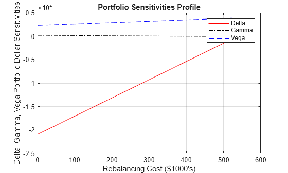
In this calling form, hedgeopt calls hedgeslf internally to determine the maximum cost needed to minimize the portfolio sensitivities and evenly samples the cost frontier.
Both hedgeopt and hedgeslf cast the optimization problem as a constrained linear least squares problem. Depending on the instruments and constraints, neither function is guaranteed to converge to a solution. In some cases, the problem space may be unbounded, and additional instrument equality constraints, or user-specified constraints, may be necessary for convergence. See Hedging with Constrained Portfolios for additional information.
See Also
Topics
- Portfolio Creation Using Functions
- Adding Instruments to an Existing Portfolio Using Functions
- Instrument Constructors
- Creating Instruments or Properties
- Searching or Subsetting a Portfolio
- Pricing a Portfolio Using the Black-Derman-Toy Model
- Pricing and Hedging a Portfolio Using the Black-Karasinski Model
- Specifying Constraints with ConSet
- Portfolio Rebalancing
- Hedging with Constrained Portfolios
- Instrument Constructors
- Hedging