Complex Burst Asynchronous Matrix Solve Using Q-less QR Decomposition
Compute the value of X in the equation A'AX = B for complex-valued matrices using asynchronous Q-less QR decomposition
Since R2022b

Libraries:
Fixed-Point Designer HDL Support /
Matrices and Linear Algebra /
Linear System Solvers
Description
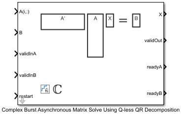
The Complex Burst Asynchronous Matrix Solve Using Q-less QR Decomposition block solves the system of linear equations A'AX = B using asynchronous Q-less QR decomposition, where A and B are complex-valued matrices.
When Regularization parameter is nonzero, the Complex Burst Asynchronous Matrix Solve Using Q-less QR Decomposition block solves the matrix equation
where λ is the regularization parameter,
A is an m-by-n matrix, and
In =
eye(n).
This block operates asynchronously. The forward- and backward-substitution and Q-less QR decomposition run independently using the latest R and B matrices.
Examples
Implement Hardware-Efficient Complex Burst Asynchronous Matrix Solve Using Q-less QR Decomposition
Implement a hardware-efficient solution to the complex-valued matrix equation A'AX=B using the Complex Burst Asynchronous Matrix Solve Using Q-less QR Decomposition block.
Ports
Input
Rows of complex matrix A, specified as a vector. A is an m-by-n matrix where m ≥ 2 and m ≥ n. If B is single or double, A must be the same data type as B. If A is a fixed-point data type, A must be signed, use binary-point scaling, and have the same word length as B. Slope-bias representation is not supported for fixed-point data types.
Data Types: single | double | fixed point
Rows of complex matrix B, specified as a vector. B is an n-by-p matrix where n ≥ 2. If A is single or double, B must be the same data type as A. If B is a fixed-point data type, B must be signed, use binary-point scaling, and have the same word length as A. Slope-bias representation is not supported for fixed-point data types.
Data Types: single | double | fixed point
Whether A(i,:) input is valid, specified as a Boolean scalar.
This control signal indicates when the data from the A(i,:) input
port is valid. When this value is 1 (true) and
the readyA value is 1 (true),
the block captures the values at the A(i,:) input port. When this
value is 0 (false), the block ignores the input
samples.
After sending a true
validInA signal, there may be some delay before
readyA is set to false. To ensure all data is
processed, you must wait until readyA is set to
false before sending another true
validInA signal.
Data Types: Boolean
Whether B input is valid, specified as a Boolean scalar. This
control signal indicates when the data from the B input port is
valid. When this value is 1 (true) and the
readyB value is 1 (true),
the block captures the values at the B input port. When this value
is 0 (false), the block ignores the input
samples.
After sending a true
validInB signal, there may be some delay before
readyB is set to false. To ensure all data is
processed, you must wait until readyB is set to
false before sending another true
validInB signal.
Data Types: Boolean
Whether to clear internal states, specified as a Boolean scalar. When this value
is 1 (true), the block stops the current calculation and clears all
internal states. When this value is 0 (false) and the value at
validIn is 1 (true), the block begins a new
subframe.
Data Types: Boolean
Output
Matrix X, returned as a matrix or vector.
Data Types: single | double | fixed point
Whether the output data is valid, specified as a Boolean scalar. This control
signal indicates when the data at output port X is valid. When this
value is 1 (true), the block has successfully computed the matrix
X. When this value is 0 (false), the output
data is not valid.
Data Types: Boolean
Whether block is ready for input A(i,:), returned as a Boolean
scalar. This control signal indicates when the block is ready for new input data. When
this value is 1 (true) and
validInA is 1 (true), the
block accepts input data in the next time step. When this value is
0 (false), the block ignores input data in the
next time step.
After sending a true
validInA signal, there may be some delay before
readyA is set to false. To ensure all data is
processed, you must wait until readyA is set to
false before sending another true
validInA signal.
Data Types: Boolean
Whether block is ready for input B, returned as a Boolean
scalar. This control signal indicates when the block is ready for new input data. When
this value is 1 (true) and
validInB is 1 (true), the
block accepts input data in the next time step. When this value is
0 (false), the block ignores input data in the
next time step.
After sending a true
validInB signal, there may be some delay before
readyB is set to false. To ensure all data is
processed, you must wait until readyB is set to
false before sending another true
validInB signal.
Data Types: Boolean
Parameters
Number of rows in matrix A, specified as a positive integer-valued scalar.
Programmatic Use
Block Parameter:
m |
| Type: character vector |
| Values: positive integer-valued scalar |
Default:
4 |
Number of columns in matrix A and rows in matrix B, specified as a positive integer-valued scalar.
Programmatic Use
Block Parameter:
n |
| Type: character vector |
| Values: positive integer-valued scalar |
Default:
4 |
Number of columns in matrix B, specified as a positive integer-valued scalar.
Programmatic Use
Block Parameter:
p |
| Type: character vector |
| Values: positive integer-valued scalar |
Default:
1 |
Regularization parameter, specified as a nonnegative scalar. Small, positive values of the regularization parameter can improve the conditioning of the problem and reduce the variance of the estimates. While biased, the reduced variance of the estimate often results in a smaller mean squared error when compared to least-squares estimates.
Programmatic Use
Block Parameter:
regularizationParameter |
| Type: character vector |
| Values: real nonnegative scalar |
Default:
0 |
Data type of the output matrix X, specified as
fixdt(1,18,14), double,
single, fixdt(1,16,0), or as a user-specified
data type expression. The type can be specified directly, or expressed as a data type
object such as Simulink.NumericType.
Programmatic Use
Block Parameter:
OutputType |
| Type: character vector |
Values:
'fixdt(1,18,14)' | 'double' |
'single' | 'fixdt(1,16,0)' |
'<data type expression>' |
Default:
'fixdt(1,18,14)' |
Algorithms
Systolic implementations prioritize speed of computations over space constraints, while burst implementations prioritize space constraints at the expense of speed of the operations. The following table illustrates the tradeoffs between the implementations available for matrix decompositions and solving systems of linear equations.
| Implementation | Throughput | Latency | Area |
|---|---|---|---|
| Systolic | High | O(nlog2(m)) | O(mn2) |
| Partial-Systolic | Medium | O(mn) | O(n2) |
| Burst | Low | O(mn) | O(n) |
Where m is the number of rows in matrix A and n is the number of columns in matrix A. Regardless of architecture, a larger word length results in lower throughput, larger latency, and larger area.
For additional considerations in selecting a block for your application, see Choose a Block for HDL-Optimized Fixed-Point Matrix Operations.
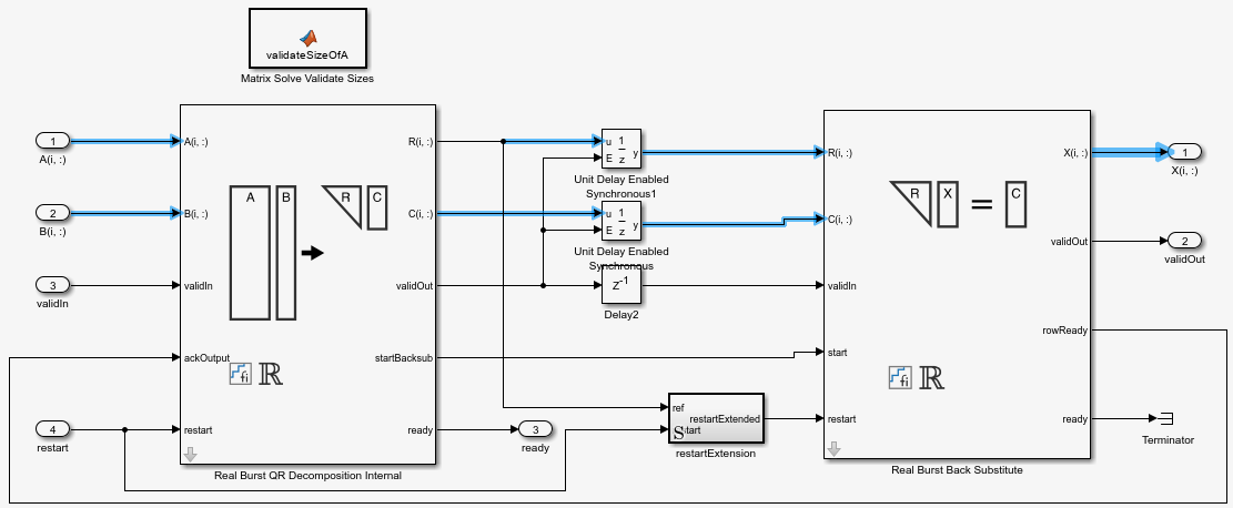
The Matrix Solve Using QR Decomposition blocks operate synchronously. These blocks first decompose the input A and B matrices into R and C matrices using a QR decomposition block. Then, a back substitute block computes RX = C. The input A and B matrices propagate through the system in parallel, in a synchronized way.

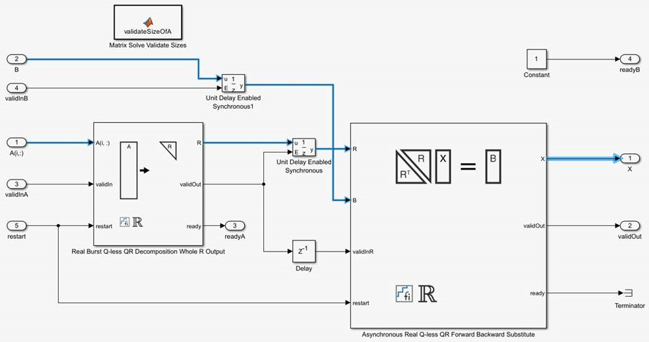
The Matrix Solve Using Q-less QR Decomposition blocks operate asynchronously. First, Q-less QR decomposition is performed on the input A matrix and the resulting R matrix is put into a buffer. Then, a forward backward substitution block uses the input B matrix and the buffered R matrix to compute R'RX = B. Because the R and B matrices are stored separately in buffers, the upstream Q-less QR decomposition block and the downstream Forward Backward Substitute block can run independently. The Forward Backward Substitute block starts processing when the first R and B matrices are available. Then it runs continuously using the latest buffered R and B matrices, regardless of the status of the Q-less QR Decomposition block. For example, if the upstream block stops providing A and B matrices, the Forward Backward Substitute block continues to generate the same output using the last pair of R and B matrices.

The Burst (Asynchronous) Matrix Solve Using Q-less QR Decomposition blocks are available in both synchronous and asynchronous operation variants, as denoted by the block name.
This block uses the AMBA AXI handshake protocol [1]. The valid/ready handshake process is used to transfer data and control information. This two-way control mechanism allows both the manager and subordinate to control the rate at which information moves between manager and subordinate. A valid signal indicates when data is available. The ready signal indicates that the block can accept the data. Transfer of data occurs only when both the valid and ready signals are high.
The Burst Asynchronous Matrix Solve Using Q-less QR Decomposition blocks accept matrix A row-by-row and matrix B as a single vector. After accepting the first valid pair of A and B matrices, the block outputs the X matrices row by row continuously. The matrix is output from the first row to the last row.
For example, assume that the input A matrix is 3-by-3. Additionally
assume that validIn asserts before ready, meaning that
the upstream data source is faster than the QR decomposition.

In the figure,
A1r1is the first row of the first A matrix,A1r2is the second row of the first A matrix, and so on.validIntoready— From a successful A row input to the block being ready to accept the next row.validOuttovalidOut— Because the Forward Backward Substitution block runs continuously, it generates output at a constant rate. This is the delay between two adjacent valid outputs.Last row
validIntovalidOut— From the last mth row input to the block starting to output the solution.This block is always ready to accept B matrices, so
readyBis always asserted.
The following table provides details of the timing for the Complex Burst Asynchronous Matrix Solve Using Q-less QR Decomposition block. Latency depends on the size of matrix A and the data types of the A and B matrices. In the table:
n is the number of columns in matrix A.
wl represents the word length of the input data in matrix A.
| Input Data Type | validIn to ready (cycles) | validOut to validOut (cycles) | Last Row validIn to validOut
(cycles) |
|---|---|---|---|
Fixed point fi | (wl*2 + 11)*n + 2 + (n + 1) | 4*n2 + 25*n + 5 + 2*n*wl + 2*n*nextpow2(wl) | 4*n2 + 25*n + 5 + 2*n*wl + 2*n*nextpow2(wl) + (wl*2 + 11)*n + n |
Scaled double fi | (wl*2 + 11)*n + 2 + (n + 1) | 4*n2 + 23*n + 5 + 2*n*wl | 4*n2 + 24*n + 5 + 2*n*wl + (wl*2 + 11)*n |
double | 118*n + 3 | 4*n2 + 21*n + 5 | 4*n2 + 139*n + 5 |
single | 60*n + 3 | 4*n2 + 21*n + 5 | 4*n2 + 81*n + 5 |
This block supports HDL code generation using the Simulink® HDL Workflow Advisor. For an example, see HDL Code Generation and FPGA Synthesis from Simulink Model (HDL Coder) and Implement Digital Downconverter for FPGA (DSP HDL Toolbox).
This example data was generated by synthesizing the block on a Xilinx® Zynq® UltraScale™ + RFSoC ZCU111 evaluation board. The synthesis tool was Vivado® v.2020.2 (win64).
The following parameters were used for synthesis.
Block parameters:
m = 16n = 16p = 1Matrix A dimension: 16-by-16
Matrix B dimension: 16-by-1
Input data type:
sfix16_En14Target frequency: 250 MHz
The following tables show the post place-and-route resource utilization results and timing summary, respectively.
| Resource | Usage | Available | Utilization (%) |
|---|---|---|---|
| CLB LUTs | 36070 | 425280 | 8.48 |
| CLB Registers | 45878 | 850560 | 5.39 |
| DSPs | 12 | 4272 | 0.28 |
| Block RAM Tile | 0 | 1080 | 0.00 |
| URAM | 0 | 80 | 0.00 |
| Value | |
|---|---|
| Requirement | 4 ns |
| Data Path Delay | 3.781 ns |
| Slack | 0.199 ns |
| Clock Frequency | 263.09 MHz |
References
[1] "AMBA AXI and ACE Protocol Specification Version E." https://developer.arm.com/documentation/ihi0022/e/
Extended Capabilities
Slope-bias representation is not supported for fixed-point data types.
HDL Coder™ provides additional configuration options that affect HDL implementation and synthesized logic.
This block has one default HDL architecture.
| General | |
|---|---|
| ConstrainedOutputPipeline | Number of registers to place at
the outputs by moving existing delays within your design. Distributed
pipelining does not redistribute these registers. The default is
|
| InputPipeline | Number of input pipeline stages
to insert in the generated code. Distributed pipelining and constrained
output pipelining can move these registers. The default is
|
| OutputPipeline | Number of output pipeline stages
to insert in the generated code. Distributed pipelining and constrained
output pipelining can move these registers. The default is
|
Supports fixed-point data types only.
Fixed-Point Conversion
Design and simulate fixed-point systems using Fixed-Point Designer™.
Version History
Introduced in R2022b
MATLAB Command
You clicked a link that corresponds to this MATLAB command:
Run the command by entering it in the MATLAB Command Window. Web browsers do not support MATLAB commands.
选择网站
选择网站以获取翻译的可用内容,以及查看当地活动和优惠。根据您的位置,我们建议您选择:。
您也可以从以下列表中选择网站:
如何获得最佳网站性能
选择中国网站(中文或英文)以获得最佳网站性能。其他 MathWorks 国家/地区网站并未针对您所在位置的访问进行优化。
美洲
- América Latina (Español)
- Canada (English)
- United States (English)
欧洲
- Belgium (English)
- Denmark (English)
- Deutschland (Deutsch)
- España (Español)
- Finland (English)
- France (Français)
- Ireland (English)
- Italia (Italiano)
- Luxembourg (English)
- Netherlands (English)
- Norway (English)
- Österreich (Deutsch)
- Portugal (English)
- Sweden (English)
- Switzerland
- United Kingdom (English)