使用 CORDIC 计算平方根

此示例说明如何在 MATLAB® 中使用 CORDIC 核算法计算平方根。基于 CORDIC 的算法对许多嵌入式应用至关重要，包括电机控制、导航、信号处理和无线通信。

CORDIC 是 COordinate Rotation DIgital Computer（坐标旋转数字计算方法）的缩写。基于吉文斯旋转的 CORDIC 算法是最节省硬件资源的算法之一，因为它只需进行迭代移位相加运算 [1,2]。CORDIC 算法不需要显式乘数，它适用于计算各种函数，如正弦、余弦、反正弦、反余弦、反正切、向量模、除法、平方根、双曲线和对数函数。

定点 CORDIC 算法需要以下操作：

每次迭代进行 1 次表查找
每次迭代进行 2 次移位
每次迭代进行 3 次加法

请注意，对于基于双曲 CORDIC 的算法，如平方根，某些迭代 ( $i = 4, 13, 40, 121, \dots, k, 3 k + 1, \dots$ ) 会重复以实现结果收敛 [2]。

使用双曲计算模式的 CORDIC 核算法

您可以使用 CORDIC 计算模式算法来计算双曲函数，如双曲三角函数、平方根、对数、幂等。

双曲向量化模式下的 CORDIC 方程

双曲向量化模式用于计算平方根。

对于向量化模式，CORDIC 方程如下：

$\begin{array}{lcl} x_{i + 1} & = & x_{i} + y_{i} \cdot d_{i} \cdot 2^{- i} \\ y_{i + 1} & = & y_{i} + x_{i} \cdot d_{i} \cdot 2^{- i} \\ z_{i + 1} & = & z_{i} - d_{i} \cdot atanh (2^{- i}) \end{array}$

其中

$i = {1, 2, 3, 4, 4, 5, \dots}$ 是每 $3 k + 1$ 次迭代会重复步骤的序列，并且

如果 $y_{i} < 0$ ，则 $d_{i} = + 1$ ，否则为 $- 1$ 。

当 $N$ 趋近于 $+ \infty$ 时，此模式提供以下结果：

$\begin{array}{lcl} x_{N} & \approx & A_{N} \sqrt{x_{0}^{2} - y_{0}^{2}} \\ y_{N} & \approx & 0 \\ z_{N} & \approx & z_{0} + atanh (y_{0} / x_{0}) \end{array}$

其中

$A_{N} = \prod_{i = {1, 2, 3, 4, 4, 5, \dots}} \sqrt{1 - 2^{- 2 i}}$ .

请注意，乘积中的序列会在每 $3 k + 1$ 个步骤中重复 [2]。

通常，会选择一个足够大的常数值作为 $N$ 的取值。因此，可以预先计算 $A_{N}$ 。

另请注意，对于平方根，仅使用 $x_{N}$ 结果。

在 MATLAB 中实现 CORDIC 双曲向量化算法

以下是 CORDIC 双曲向量化核算法的 MATLAB 代码实现示例（对于标量 x、y 和 z 的情况）。以下代码可同时用于定点和浮点数据类型。

CORDIC 双曲向量化核

k = 4; % Used for the repeated (3*k + 1) iteration steps
for idx = 1:N
    xtmp = bitsra(x, idx); % multiply by 2^(-idx)
    ytmp = bitsra(y, idx); % multiply by 2^(-idx)
    if y < 0
        x(:) = x + ytmp;
        y(:) = y + xtmp;
        z(:) = z - atanhLookupTable(idx);
    else
        x(:) = x - ytmp;
        y(:) = y - xtmp;
        z(:) = z + atanhLookupTable(idx);
    end
    if idx==k
        xtmp = bitsra(x, idx); % multiply by 2^(-idx)
        ytmp = bitsra(y, idx); % multiply by 2^(-idx)
        if y < 0
            x(:) = x + ytmp;
            y(:) = y + xtmp;
            z(:) = z - atanhLookupTable(idx);
        else
            x(:) = x - ytmp;
            y(:) = y - xtmp;
            z(:) = z + atanhLookupTable(idx);
        end
        k = 3*k + 1;
    end
end % idx loop

双曲反正切查找表 atanhLookupTable 定义如下，在代码生成中将预先计算它并成为常量。

atanhLookupTable = cast(atanh(2.^-(1:N)),'like',z);

使用 CORDIC 双曲向量化核计算平方根

明智选择的初始值允许 CORDIC 核双曲向量化模式算法计算平方根。

首先，执行以下初始化步骤：

将 $x_{0}$ 设置为 $v + 0.25$ 。
将 $y_{0}$ 设置为 $v - 0.25$ 。

在 $N$ 次迭代后，随着 $N$ 逼近 $+ \infty$ ，这些初始值会导致以下输出：

$x_{N} \approx A_{N} \sqrt{(v + 0.25)^{2} - (v - 0.25)^{2}}$

这可以进一步简化如下：

$x_{N} \approx A_{N} \sqrt{v}$

其中 $A_{N}$ 是如上定义的 CORDIC 增益。

请注意，对于平方根， $z$ 和 atanhLookupTable 对结果不起作用。因此，未使用 $z$ 和 atanhLookupTable。

CORDIC 平方根核的 MATLAB 实现

以下是 CORDIC 平方根核算法的 MATLAB 代码实现示例（对于标量 x 和 y 的情况）。以下代码可同时用于定点和浮点数据类型。

CORDIC 平方根核

k = 4; % Used for the repeated (3*k + 1) iteration steps
for idx = 1:N
    xtmp = bitsra(x, idx); % multiply by 2^(-idx)
    ytmp = bitsra(y, idx); % multiply by 2^(-idx)
    if y < 0
        x(:) = x + ytmp;
        y(:) = y + xtmp;
    else
        x(:) = x - ytmp;
        y(:) = y - xtmp;
    end
    if idx==k
         xtmp = bitsra(x, idx); % multiply by 2^(-idx)
         ytmp = bitsra(y, idx); % multiply by 2^(-idx)
         if y < 0
             x(:) = x + ytmp;
             y(:) = y + xtmp;
         else
             x(:) = x - ytmp;
             y(:) = y - xtmp;
         end
         k = 3*k + 1;
      end
 end % idx loop

以下代码与上述 CORDIC 双曲向量化核实现相同，只是未使用 z 和 atanhLookupTable。这样，每次迭代都省去 1 次表查找和 1 次加法运算。

示例

使用 cordicsqrt 函数，通过十次 CORDIC 核迭代计算 v_fix 的近似平方根。

step  = 2^-7;
v_fix = fi(0.5:step:(2-step), 1, 20); % fixed-point inputs in range [.5, 2)
niter = 10; % number of CORDIC iterations
x_sqr = cordicsqrt(v_fix, niter);

获取 CORDIC 输出的真实值 (RWV) 以进行比较，并绘制 MATLAB 参考值与 CORDIC 平方根值之间的误差。

x_cdc = double(x_sqr); % CORDIC results (scaled by An_hp)
v_ref = double(v_fix); % Reference floating-point input values
x_ref = sqrt(v_ref);   % MATLAB reference floating-point results
figure;
subplot(211);
plot(v_ref, x_cdc, 'r.', v_ref, x_ref, 'b-');
legend('CORDIC', 'Reference', 'Location', 'SouthEast');
title('CORDIC Square Root (In-Range) and MATLAB Reference Results');
subplot(212);
absErr = abs(x_ref - x_cdc);
plot(v_ref, absErr);
title('Absolute Error (vs. MATLAB SQRT Reference Results)');

Figure contains 2 axes objects. Axes object 1 with title CORDIC Square Root (In-Range) and MATLAB Reference Results contains 2 objects of type line. One or more of the lines displays its values using only markers These objects represent CORDIC, Reference. Axes object 2 with title Absolute Error (vs. MATLAB SQRT Reference Results) contains an object of type line.

克服算法输入范围限制

许多平方根算法将输入值 $v$ 归一化到 [0.5, 2) 范围内。这种预处理通常使用固定字长归一化完成，可用于支持小输入值范围和大输入值范围。

基于 CORDIC 的平方根算法实现对超出此范围的输入特别敏感。cordicsqrt 函数通过基于以下数学关系的归一化方法克服此算法范围限制：

$v = u \cdot 2^{n}$ （适用于某些 $0.5 < = u < 2$ 和某些偶数 $n$ ）。

因此：

$\sqrt{v} = \sqrt{u} \cdot 2^{n / 2}$

在 cordicsqrt 函数中，上述 $u$ 和 $n$ 的值是在输入 $v$ 的归一化过程中找到的。 $n$ 是输入 $v$ 的二进制表示中前导零最高有效位 (MSB) 的数量。这些值是通过一系列按位逻辑和移位运算找到的。请注意，因为 $n$ 必须为偶数，如果前导零 MSB 的数量为奇数，则会进行一次额外的位移以使 $n$ 为偶数。这些移位后的结果值是值 $0.5 < = u < 2$ 。

$u$ 成为基于 CORDIC 的平方根核的输入，会在此处计算 $\sqrt{u}$ 的逼近。然后按 $2^{n / 2}$ 对结果进行缩放，使其回到正确的输出范围。这通过简单的按 $n / 2$ 位移位来实现。移位方向（左或右）取决于 $n$ 的符号。

示例

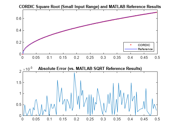
使用 CORDIC 计算具有小的非负范围的 10 位定点输入数据的平方根。在相同输入范围内，将基于 CORDIC 的算法结果与浮点 MATLAB 参考结果进行比较。

step     = 2^-8;
u_ref    = 0:step:(0.5-step); % Input array (small range of values)
u_in_arb = fi(u_ref,0,10);    % 10-bit unsigned fixed-point input data values
u_len    = numel(u_ref);
sqrt_ref = sqrt(double(u_in_arb)); % MATLAB sqrt reference results
niter    = 10;
results  = zeros(u_len, 2);
results(:,2) = sqrt_ref(:);

计算等效真实值 (RWV) 结果。绘制 CORDIC 和 MATLAB 参考结果的 RWV。

x_out = cordicsqrt(u_in_arb, niter);
results(:,1) = double(x_out);
figure;
subplot(211);
plot(u_ref, results(:,1), 'r.', u_ref, results(:,2), 'b-');
legend('CORDIC', 'Reference', 'Location', 'SouthEast');
title('CORDIC Square Root (Small Input Range) and MATLAB Reference Results');
axis([0 0.5 0 0.75]);
subplot(212);
absErr = abs(results(:,2) - results(:,1));
plot(u_ref, absErr);
title('Absolute Error (vs. MATLAB SQRT Reference Results)');

Figure contains 2 axes objects. Axes object 1 with title CORDIC Square Root (Small Input Range) and MATLAB Reference Results contains 2 objects of type line. One or more of the lines displays its values using only markers These objects represent CORDIC, Reference. Axes object 2 with title Absolute Error (vs. MATLAB SQRT Reference Results) contains an object of type line.

示例

使用 CORDIC 计算具有大的正范围的 16 位定点输入数据的平方根。在相同输入范围内，将基于 CORDIC 的算法结果与浮点 MATLAB 参考结果进行比较。

u_ref    = 0:5:2500;       % Input array (larger range of values)
u_in_arb = fi(u_ref,0,16); % 16-bit unsigned fixed-point input data values
u_len    = numel(u_ref);
sqrt_ref = sqrt(double(u_in_arb)); % MATLAB sqrt reference results
niter    = 16;
results  = zeros(u_len, 2);
results(:,2) = sqrt_ref(:);

计算等效真实值 (RWV) 结果。绘制 CORDIC 和 MATLAB 参考结果的 RWV。

x_out = cordicsqrt(u_in_arb, niter);
results(:,1) = double(x_out);
figure;
subplot(211);
plot(u_ref, results(:,1), 'r.', u_ref, results(:,2), 'b-');
legend('CORDIC', 'Reference', 'Location', 'SouthEast');
title('CORDIC Square Root (Large Input Range) and MATLAB Reference Results');
axis([0 2500 0 55]);
subplot(212);
absErr = abs(results(:,2) - results(:,1));
plot(u_ref, absErr);
title('Absolute Error (vs. MATLAB SQRT Reference Results)');

Figure contains 2 axes objects. Axes object 1 with title CORDIC Square Root (Large Input Range) and MATLAB Reference Results contains 2 objects of type line. One or more of the lines displays its values using only markers These objects represent CORDIC, Reference. Axes object 2 with title Absolute Error (vs. MATLAB SQRT Reference Results) contains an object of type line.

参考资料

Jack E. Volder, "The CORDIC Trigonometric Computing Technique," IRE Transactions on Electronic Computers, Volume EC-8, September 1959, pp. 330-334.
J.S. Walther, "A Unified Algorithm for Elementary Functions," Conference Proceedings, Spring Joint Computer Conference, May 1971, pp. 379-385.

另请参阅

CORDIC Square Root HDL Optimized