Introduction to Class Fusion and Classification-Aided Tracking

Introduction

Detections generated from regular sensors usually contain kinematic information of the targets, such as measurement and measurement noise. Some sensors also have the capability of identifying class of targets and outputting target classification labels. In the Sensor Fusion and Tracking Toolbox, you represent detections in the form of objectDetection objects. With the objectDetection object, you specify kinematic information by using the Measurement, MeasurementNoise, and MeasurementParameters properties. Meanwhile, you can specify classification information by using the ObjectClassID and ObjectClassParameters properties. See the Convert Detections to objectDetection Format example for how to use the objectDetection object to create detections.

In most cases, a classifier outputs the classes of detections based on a fixed set of possible labels. For example, {ClassA, ClassB, ..., ClassZ}. A classifier usually outputs the classification results in one of the three formats [1]:

You can always convert a Soft or Ranked output to a Crisp output by selecting the most likely class. The Sensor Fusion and Tracking Toolbox uses the Crisp representation.

Class Fusion

In the context of object tracking, you can use class fusion for two main objectives. First, maintain and improve the class estimation for each tracked object over time. Second, fuse different and possibly conflicting classification results that are assigned to the same object.

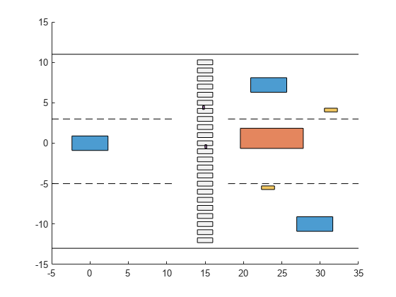
In this example, consider the 4 following classes 'Car', 'Truck', 'Bicycle', and 'Pedestrian' as well as a simple traffic crosswalk scenario. In the scenario, two pedestrians are walking on the crosswalk, whereas a truck and two other cars stop on the right side of the crosswalk. Additionally, two bicycles are in between the truck and the cars. The ego vehicle is located at coordinates [0, 0]. Use the helperClassFusionDisplay class to visualize the scenario.

helperClassFusionDisplay.plotClassFusionScene();

The ego vehicle is equipped with two vision detectors (camera paired with a classifier). Each vision detector provides detections with a crisp classification. The two vision detectors have different classification accuracies, represented by their respective confusion matrices, normalized by row.

${\mathit{C}}_1=\left[\begin{array}{cccc}0.90& 0.05& 0.03& 0.02\\ 0.05& 0.90& 0.03& 0.02\\ 0.20& 0.20& 0.30& 0.30\\ 0.20& 0.20& 0.30& 0.30\end{array}\right]$ and ${\mathit{C}}_2=\left[\begin{array}{cccc}0.30& 0.20& 0.02& 0.02\\ 0.05& 0.30& 0.03& 0.03\\ 0.02& 0.03& 0.90& 0.05\\ 0.02& 0.03& 0.05& 0.90\end{array}\right]$

The first confusion matrix denotes that if the true class of a target is 'Truck' the classifier classifies the detection 90% of the time as a 'Truck', 5% of the time as 'Car', 3% of the time as bicycle, and finally 2% of the time as a pedestrian. Therefore, the first detector performs well when classifying Trucks and Cars but performs poorly when classifying bicycles and pedestrians. The second detector, on the contrary, is more accurate on 'Bicycles' and 'Pedestrians' classification.

Load the synthetic vision detection data into the workspace. For each vision detector, inspect the confusion matrix saved in the ObjectClassParameters property of the first objectDetection object at the first time step.

load("visionDetectionLog.mat", "datalog");
disp(datalog(1).Detections1{1}.ObjectClassParameters.ConfusionMatrix);

    0.9000    0.0500    0.0300    0.0200
    0.0500    0.9000    0.0300    0.0200
    0.2000    0.2000    0.3000    0.2000
    0.2000    0.2000    0.3000    0.3000

disp(datalog(1).Detections2{1}.ObjectClassParameters.ConfusionMatrix);

    0.3000    0.2000    0.2000    0.2000
    0.2000    0.3000    0.2000    0.2000
    0.0300    0.0200    0.9000    0.0500
    0.0300    0.0200    0.0500    0.9000

To fuse the detections across time, create a trackerJPDA object and set the ClassFusionMethod property to "Bayes". Also set the InitialClassProbabilities property to model an environment with a uniform a priori distribution of classes.

globalTracker = trackerJPDA(ClassFusionMethod="Bayes",...
    InitialClassProbabilities=[0.25 0.25 0.25 0.25]);

Clone the tracker twice for tracking with each individual detector.

localTracker1 = clone(globalTracker);
localTracker2 = clone(globalTracker);

Simulate the tracking process and visualize the results using the helperClassFusionDisplay helper class

display = helperClassFusionDisplay();

for i=1:numel(datalog)

    time = datalog(i).Time;
    dets1 = datalog(i).Detections1;
    dets2 = datalog(i).Detections2;

    tracks = globalTracker([dets1; dets2], time);
    tracks1 = localTracker1(dets1, time);
    tracks2 = localTracker2(dets2, time);

    update(display, dets1, dets2, tracks, tracks1, tracks2);
end

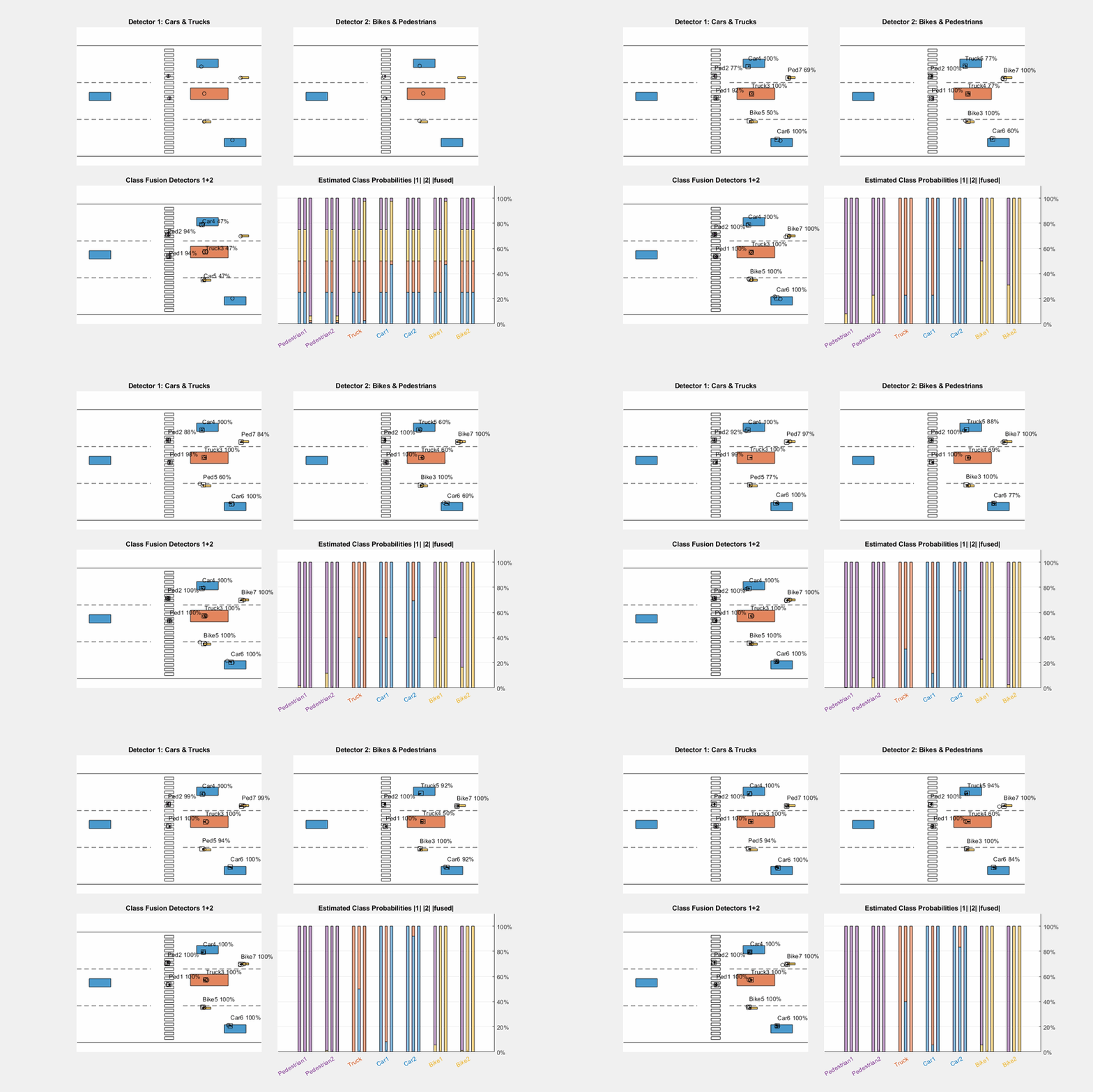
The GIF below shows the recorded animation of the scene.

The top left tile shows the tracking result based only on the detections from the first detector. From its confusion matrix, this detector provides accurate classification for cars and trucks, which allows the class estimation algorithms to accurately predict the classes of the two cars and the truck. However, this detector poorly classifies bicycles, which leads to wrong classifications for the two bicycles.

The top right tile shows the tracking result based only on detections from the second detector. In this case, all the pedestrians and bicycles are correctly classified.

The bottom left tile shows the results obtained when fusing detections from the two detectors. The high confidence of the first detector in classifying cars and trucks combined with the high confidence of the second detector in classifying pedestrians and bicycles provides optimal results.

The bar chart on the bottom right tile shows the class probability distributions for each target. The class probabilities for each target are stacked in a column. For each object, the left column corresponds to the first detector, the middle column corresponds to the second detector, and the right column corresponds to fused results from both detectors. At the end of the simulation, you see that each target is correctly estimated with 100% probability by the fusion of the two detectors.

Classification-Aided tracking

In this section, you explore a scenario in which measurement-to-track association benefits from classification data. This is often referred to as classification-aided tracking. Tracking closely spaced targets that move in similar patterns is difficult because noisy kinematic measurements can have comparable likelihoods to be associated to the same target. This example uses the scenario proposed in [2], in which six targets fly in formation. Assume that there are four different target classes in total and that the six targets belong to class Class1, Class2, Class3, Class4, Class3, and Class4, respectively.

Load the classification-aided tracking scenario data from a MAT-file and inspect the confusion matrix.

load('classAidedScenarioData.mat','scenario','allData');
disp(allData(1).Detections{1}.ObjectClassParameters.ConfusionMatrix);

    0.8500    0.0500    0.0500    0.0500
    0.0500    0.8500    0.0500    0.0500
    0.0500    0.0500    0.8500    0.0500
    0.0500    0.0500    0.0500    0.8500

From the confusion matrix, the classifier classifies correctly 85% of the time and misclassification are equiprobable.

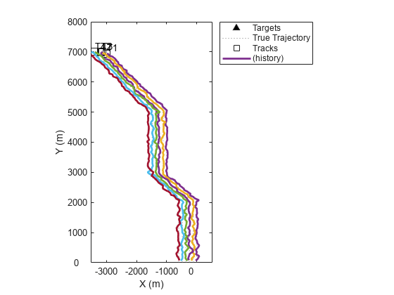
Next, use a helper class to visualize the trajectories of the six targets. The targets are closely spaced and kinematic ambiguity of measurements is unavoidable.

helperClassAidedTrackingDisplay.plotClassAidedScene(scenario);

Configure a tracker with a default interacting multiple model (IMM filter) because the targets perform maneuvers in the scenario. Set the ClassFusionMethod property to "Bayes" and the InitialClassProbabilities property to the known distribution of target classes in the scenario. You choose the global nearest neighbor (GNN) tracker to avoid track coalescence.

gnn = trackerGNN(AssignmentThreshold = 100,...
    MaxNumTracks=10,...
    FilterInitializationFcn="initekfimm",...
    ClassFusionMethod="Bayes",...
    InitialClassProbabilities = [0.2 0.2 0.3 0.3]);

The ClassFusionWeight property defines how the tracker combines the kinematic and classification costs to obtain the overall data association cost.

The tracker then uses the assignment algorithm, specified by the Assignment property, to calculate the optimal assignment between detections and tracks based on the $\mathrm{OverallCost}$. The ClassFusionWeight property ranges from 0 (kinematics only) to 1 (classification only). Move the slider control below to observe how the tracking performance varies with the weight change.

gnn.ClassFusionWeight = 0.7;

Simulate the tracking process, save the information analysis output from the tracker, and visualize the tracking results.

display2 = helperClassAidedTrackingDisplay(scenario);
infoLog = cell(1,numel(allData));
tracks = objectTrack.empty;

for i=1:numel(allData)

    time = allData(i).Time;
    dets = allData(i).Detections;

    % Update tracker
    [tracks, ~,~, info] = gnn(dets,time);

    update(display2, tracks);
    % Store info log
    infoLog{i} = info;
end

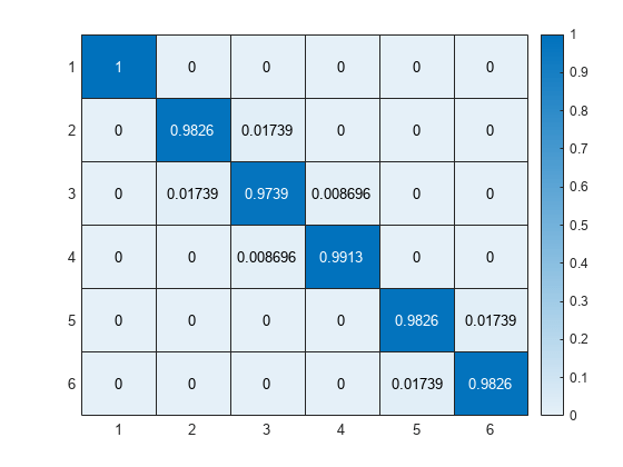
You can use a purity matrix plot to assess the data association performance in this scenario. In the purity matrix, the (i,j) entry represents the percentage of detections that originate from the true target j assigned to the estimated track i. A tracking algorithm with perfect association would lead to an identity purity matrix. The further away the main values are from the matrix diagonal, the worse the association is. Note that early track swap, can result in a purity matrix with main values on the secondary diagonal. This, however, still indicates a good data association. You can see such a case by setting ClassFusionWeight property to 0.6.

plotPurityMatrix(display2,infoLog)

Note that for this example, the best results are obtained for a value of 0.7. It is expected that using only kinematics will lead to poor tracking because of the nature of the scenario. However, relying only on classification is not a good option either, because any misclassification can result in false association and the kinematics must contribute in data association.

Conclusion

In this example you learned how to configure the trackerGNN and the trackerJPDA objects to fuse classified detections with a Bayesian Product class fusion algorithm. Class fusion that operates on crisp classifications with the knowledge of the confusion matrix allows you to estimate the probability of track classes. In the second part, you use classification information to improve data association in an ambiguous scenario. You learned balancing the kinematics and classification association costs can refine the overall tracking performance.

References

[1] Kuncheva, Ludmila. Fuzzy classifier design. Vol. 49. Springer Science & Business Media, 2000.

[2] Bar-Shalom, Yaakov, Thia Kirubarajan, and Cenk Gokberk. "Tracking with classification-aided multiframe data association." IEEE Transactions on Aerospace and Electronic systems 41, no. 3 (2005): 868-878.