Introduction to PHD Filter

Open Live Script

This example introduces the principles behind the probability hypothesis density (PHD) filter and how it can be used to estimate the number and states of multiple objects in a scene. The PHD filter is a type of filter derived using a random finite set (RFS) framework for object tracking.

PHD Fundamentals

In this section, you will learn about the definition of the PHD, its properties, and the fundamental concepts behind the PHD filter.

The PHD is a function defined over the state-space. It is often denoted as $D (x)$ , where $x$ is a state in the state space. The output of this function is a scalar real value, which describes the expected number of targets per unit volume of the state-space at $x$ . Therefore, the expected number of objects in a small region $dx$ around $x$ can be described as $D (x) dx$ . The total number of expected objects in the entire scene can be obtained by integrating the PHD over the entire state-space, as follows:

$N_{e} =$

$\int D (x) d x$

Similar to how the mean or average is defined for any type of single-object probability density function (PDF) such as Gaussian, Gaussian mixture, or set of particles, the PHD is defined over any type of multi-object pdf such as Poisson, multi-Bernoulli, and so on. When the multi-object PDF is approximated using Poisson, the PDF for the RFS defining the targets as $X = {x_{1}, x_{2}, x_{3} . . . x_{n}}$ is fully defined by PHD function, $D (x)$ .

$p (X) = e^{- N_{e}} D (x_{1}) D (x_{2}) . . . D (x_{n})$

The PHD filter, as the name suggests, is an algorithm which recursively estimates the PHD. The PHD filter is derived using multi-object recursive Bayesian estimator and thus has two steps; a prediction step, and a correction step.

$D_{0} (x) . . . \to D_{k - 1 | k - 1} (x) \to D_{k | k - 1} (x) \to D_{k | k} (x) . . . \to D_{L | L} (x)$

The subscript $k | k - 1$ describes the predicted PHD and the subscript $k | k$ defines the updated PHD using measurement set $Z_{k}$ . Standard equations exist to describe the prediction and correction of the PHD under Poisson clutter model. These equations define the recursion of PHD function under arbitrary forms of the PHD function. However, to define closed-form recursions for the PHD, the PHD function must be approximated with a family of distributions that can be described with some parameters. The most common form of this approximation is the Gaussian-mixture PHD (GM-PHD), which describes the PHD as Gaussian mixture with a defined number of components ( $J_{k | k}$ ), their weights ( $w_{k | k}^{i}$ ), means ( $m_{k | k}^{i}$ ), and covariances ( $P_{k | k}^{i}$ ). Note that the number of components in the mixture varies with time.

$D_{k | k} (x) = \sum_{i = 1}^{J_{k | k}} w_{k | k}^{i} N (x, m_{k | k}^{i}, P_{k | k}^{i})$

Using this form of the PHD, the prediction and update of the PHD can be defined by formulating the prediction and update of the number of components and their weights, means, and covariances. In the next two sections, you will learn about the closed-form recursion of the GM-PHD filter during the prediction and update steps.

PHD Prediction

In this section, you will learn about the prediction step of the GM-PHD filter. The predicted PHD can be described using a superposition of two functions.

$D_{k | k - 1} (x) = D_{k | k - 1, s} (x) + D_{k, b} (x)$

where $D_{k | k - 1, s} (x)$ describes the PHD of targets which survived from last step and the $D_{k, b} (x)$ describes the PHD of the targets which appeared since the last step. Both $D_{k | k - 1, s} (x)$ and $D_{k, b} (x)$ are Gaussian mixtures in the GM-PHD filter. The PHD of surviving targets, $D_{k | k - 1, s} (x)$ , for GM-PHD can be calculated by using the following closed-form recursion on $D_{k - 1 | k - 1} (x)$

Reduce the weight of each Gaussian component by using a survival probability ( $P_{s}$ )
Update the mean and covariance of each component using a linear Gaussian model.

The standard GM-PHD prediction assumes a linear, Gaussian motion model and a constant probability of survival. However, approximate techniques such as extended or unscented transforms can be used in practice for non-linear models. Similarly, a different survival probability for each component can be used in practice. The image below shows the prediction step of the PHD with three components in the Gaussian mixture. Note that after prediction, the number of components in the PHD is increased by the number of birth components.

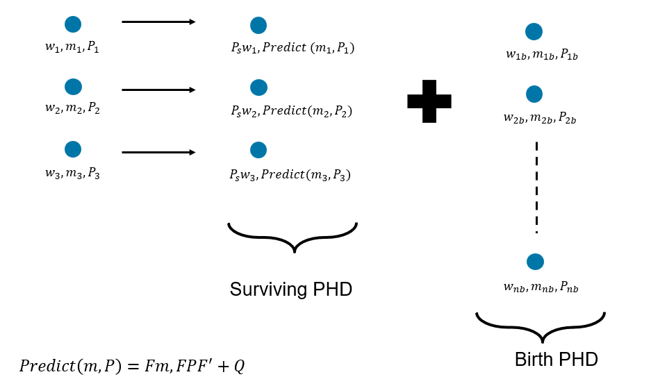
The Gaussian mixture describing the PHD of newly born targets can be provided using two main methods. In the first method, the weights, means, and covariances of each Gaussian component are preselected using prior information. This can be described as a predictive PHD birth model. In the second method, the weights, means, and covariances of each Gaussian component are determined using the measurements by using an inverse measurement model. This can be described as an adaptive PHD birth model. A combination of both techniques can also be used in practice. Note that the sum of weights of the Gaussian mixture used for the birth PHD represents the expected number of targets born during prediction.

PHD Update

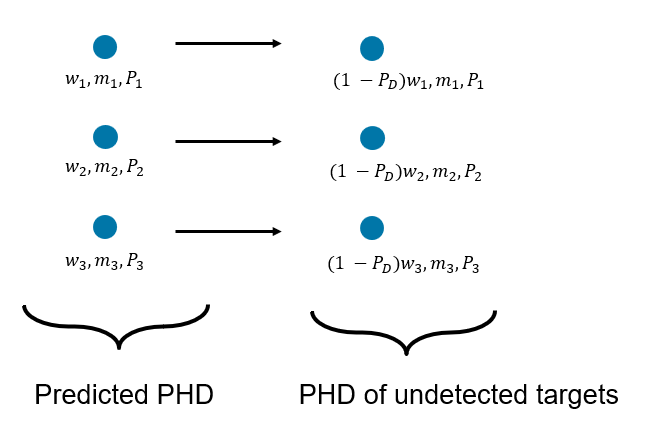
In this section, you will learn about the correction or update step of the GM-PHD filter. The corrected PHD describes the PHD of the target RFS at time step k by updating the predicted PHD with the measurement set collected at this step, $Z_{k}$ . Similar to the predicted PHD, the corrected PHD can also be described as a superposition of two PHD functions.

$D_{k | k} (x) = D_{k | k, u} (x) + D_{k | k, d} (x)$

Here $D_{k | k, d} (x)$ describes the PHD of the detected targets and $D_{k | k, u} (x)$ describes the PHD of undetected targets at step k. The PHD of undetected targets for GM-PHD is calculated by simply scaling the weights using a probability of detection, $P_{D}$ . The standard GM-PHD update uses a constant probability of detection. However, approximate techniques can be employed by using a different detection probability value for each component.

The PHD of detected targets can be formulated by using individual measurements in the set $Z_{k} = {z_{1,} z_{2}, . . ., z_{M}}$ . For each measurement and each component in the predicted PHD, a scaling term $L_{ij}$ is calculated to update the weights. The mean and covariance of each component is updated by using a Kalman filter-like correction on each component with each measurement. The standard GM-PHD filter uses a linear, Gaussian measurement model. However, approximations using extended or unscented correction can be used in practice to account for non-linear models. The image below shows the update step with three components in the predicted PHD.

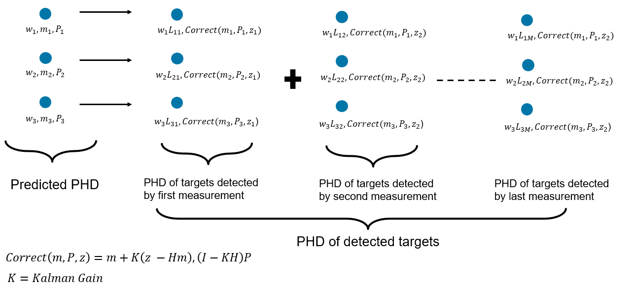
Another way to illustrate the PHD update is by grouping the updated components with respect to original components in the predicted PHD. Each component in the Gaussian mixture goes through M + 1 transformations, where M is the number of measurements. This tree form of the PHD update is informative to understand that the PHD filter considers uncertainty in data association.

For a linear, Gaussian measurement model and using point target assumptions (one detection per object), the scaling term $L_{ij}$ is computed as:

$L_{ij} = \frac{P_{D} q_{ij}}{K_{c} + P_{D} \sum_{i = 1}^{J_{k + 1 | k}} w_{i} q_{ij}}$

$q_{ij} = N (z_{j}, {Hm}_{i}, {HP}_{i} H^{'} + R)$

where $P_{D}$ and $K_{c}$ defines the detection probability and clutter density of the sensor. Note that the $q_{ij}$ represents the standard association likelihood between a measurement and a Gaussian pdf used by data association based trackers. Also note that PHD filter provides equations for updated weights of each component in the Gaussian mixture without enumerating over data association hypothesis. The PHD update results in an increase of components in the Gaussian mixture. Specifically, if the predicted PHD has N components and there are M measurements from the sensor, then the corrected PHD has N*(M+1) components. With every recursion, the number of components defining the PHD grow substantially. In order to maintain the computational efficiency of the PHD filter, techniques like merging and pruning of components are necessary.

For extended target measurement model (more than one detection per object), the PHD update is repeated for each possible partition of the measurements. In addition, the scaling terms per partition are further scaled down by a partition probability. For more details about extended target PHD recursion, refer to [2].

PHD Visualization For Scalar State Estimation

In the previous sections, you learned about the PHD prediction and update steps using the PHD filter. In this section, you will use the PHD filter in MATLAB® to predict, update, and visualize the PHD during each step. You use the filter to estimate the state of the objects described by a scalar state, $x$ = $p_{x}$ , denoting their position in the X coordinate. You use this simplistic state space definition to allow visualizing the PHD as a function of state-space. However, the concepts discussed here apply to higher dimensional state-spaces such as 3-D position, velocity of the objects.

The motion model of the target is described as:

$x_{k + 1} = x_{k} + w_{k}$

where $w_{k}$ is the process noise, defined as zero-mean while noise with variance 0.25.

stateTransitionFcn = @(x, dT)x;
hasAdditiveProcessNoise = true;
Q = 0.25;

The measurement model of the sensor is described as:

$z_{k} = x_{k} + v_{k}$

where $v_{k}$ is the measurement noise, defined as zero-mean while noise with variance 1.

measurementFcn = @(x)x;
hasAdditiveMeasurementNoise = true;
R = 1;

You use a predictive birth model with 8 Gaussian components, each with a weight of 0.01. You sample the means of these Gaussian components linearly between -40 and 40 and set their variance to 16.

mb = linspace(-40,40,8);
Pb = 16*ones(1,1,8);
wb = 0.01*ones(1,8);

You assume that the sensor detection probability is 0.9, the survival probability between two steps is 0.99, and the clutter density of the sensor is 1e-2.

Pd = 0.9;
Ps = 0.99;
Kc = 1/100;

You start the recursion with PHD containing zero components.

m0 = zeros(1,0);
P0 = zeros(1,1,0);
w0 = zeros(1,0);

You use the gmphd filter object to describe the PHD components and motion, measurement models. gmphd class provides necessary building blocks to formulate the prediction and correction steps of the GM-PHD filter.

% Create PHD object to describe PHD of the targets
phd = gmphd(m0,P0,...
    'Weights',w0,...
    'StateTransitionFcn',stateTransitionFcn,...
    'HasAdditiveProcessNoise',hasAdditiveProcessNoise,...
    'ProcessNoise',Q,...
    'MeasurementFcn',measurementFcn,...
    'HasAdditiveMeasurementNoise',hasAdditiveMeasurementNoise);

% Create PHD object to describe birth PHD. No need to specify state
% transition etc. functions. You set the MaxNumComponents to 8 to specify
% the maximum memory required by this object.
birthPHD = gmphd(mb,Pb,'Weights',wb,'MaxNumComponents',8);

Run one iteration of PHD prediction. This is achieved with three steps using the gmphd object. First, you use the predict method of the filter to predict the mean and covariance of the each existing component. Second, you use the scale method to reduce the weights to Gaussian components to model the impact of survival probability on the PHD function. Lastly, you use the append method to add the PHD of the birth targets to the PHD.

% Predict existing components mean and covariances
predict(phd, 1);

% Scale by survival probability
scale(phd, Ps);

% Add birth PHD
append(phd, birthPHD);

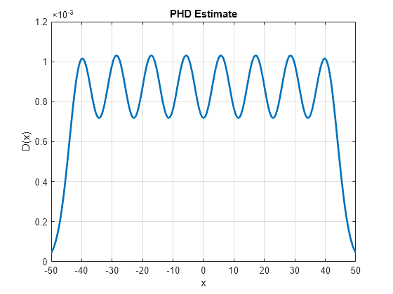
To visualize the PHD, you calculate the value of the PHD function over the range -50 to 50 sampled with a resolution of 0.1. To calculate the PHD at a given state, you use the Gaussian-mixture formula using the supporting function, calculatePHD. Notice that the PHD plot shows the Gaussian mixture birth model used in this example.

% Vector over which PHD is visualized
x = -50:0.1:50;

% Compute the value of the PHD function
D = arrayfun(@(e)calculatePHD(phd, e),x);

% Plot the PHD
h = plot(x,D,'LineWidth',2);
xticks(-50:10:50);
xlabel('x'); 
ylabel('D(x)')
grid on;
title('PHD Estimate')

At this step, you assume that the sensor reports three measurements at z = -23.8, z = -12.5, and z = 29.3. The first two measurements represent measurements from true target and the third measurement represents a clutter measurement. You assemble these measurements using objectDetection.

Z1 = cell(3,1);
Z1{1} = objectDetection(1,-23.8,'MeasurementNoise',R);
Z1{2} = objectDetection(1,-12.5,'MeasurementNoise',R);
Z1{3} = objectDetection(1,29.4,'MeasurementNoise',R);

Run one iteration of the PHD correction. First, you calculate the PHD of undetected targets. For point target models, this is simply achieved by scaling the weights of the PHD components with the probability of being undetected.

phdUndetected = clone(phd);
scale(phdUndetected, 1 - Pd);

To calculate the PHD of detected targets, you use three steps. First, you use the likelihood method of the filter to obtain the $qij$ terms defined above. This represents the log-likelihood of association as described in the PHD update description. Second, you use supporting function calculateScaling, which uses the point target assumptions computes the scaling terms $L_{ij}$ for correction using log computations. Using logarithmic format of the likelihood is often necessary to preserve numerical accuracy. Lastly, you use the correct method of the filter to update the PHD of detected targets.

% Inform PHD filter about detections at current step
phd.Detections = Z1;

% Use the likelihood to compute qij against each detection in the
% phd.Detections. 
detectionGroups = eye(3,'logical'); 
logqij = likelihood(phd, detectionGroups);

% Compute scaling term using point-object assumption
Lij = calculateScaling(logqij, phd.Weights, Pd, Kc);

% Update the PHD filter
correct(phd, detectionGroups, Lij);

To complete the update step, you add the PHD of undetected targets to the PHD of detected targets to obtain the final updated PHD.

append(phd, phdUndetected);

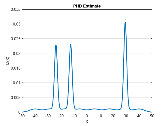
You visualize the updated PHD function over the region defined earlier. Notice that the PHD function shows peaks at the measurements observed in this step. However, the value of the PHD is still small denoting that the filter is not yet sure if there is a true object at those locations.

% Compute the value of the PHD function
D = arrayfun(@(x)calculatePHD(phd, x),x);
h.YData = D;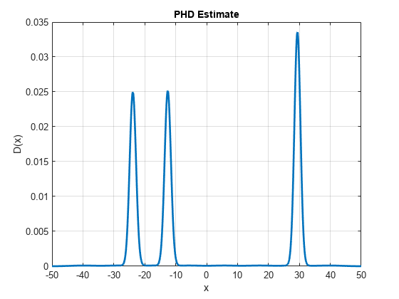

Run another prediction step and visualize the PHD function. The iteration is wrapped in a helper function, runPredictionIteration, defined in the script below. Notice that three main events happened to the PHD plot during prediction. First, the peak values of the PHD decreased due to the impact of survival probability. Second, the peaks widened a little bit due to the impact of process noise. And lastly, you see smaller peaks denoting the newly born targets modeled using the birth process.

runPredictionIteration(phd, birthPHD, Ps);
D = arrayfun(@(e)calculatePHD(phd,e),x);
h.YData = D;

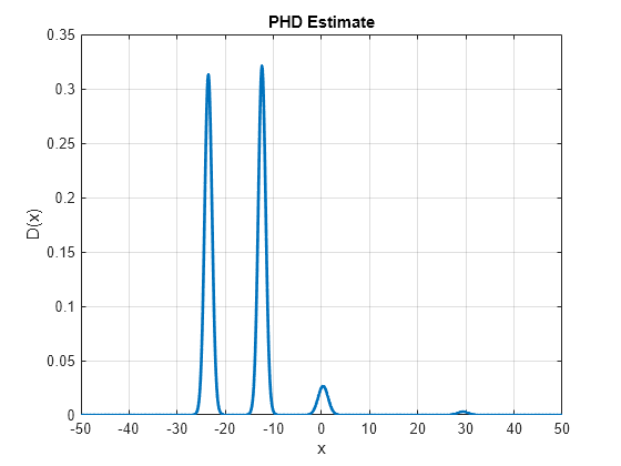
Run another correction step. At this step, you assume that the sensor again observes three measurements at z = 0.3, z = -12.25, and z = -23.28. The first measurement represents the clutter measurement. Notice that the PHD after correction shows much more distinct peaks near true target measurements, a diminished the peak from clutter measurement at the last step and a new peak at the new clutter measurement at z = 0.3. Also notice that the peak near the new clutter measurement is much smaller as compared to the peak near the true targets. This is because the PHD filter is more confident about the presence of true objects in that region.

% Assemble detections at step 2
Z2 = cell(3,1);
Z2{1} = objectDetection(2,-23.28,'MeasurementNoise',R);
Z2{2} = objectDetection(2,-12.25,'MeasurementNoise',R);
Z2{3} = objectDetection(2,0.3,'MeasurementNoise',R);

% Run PHD correction
runCorrectionIteration(phd, Z2, Pd, Kc)

% Update the PHD plot
D = arrayfun(@(e)calculatePHD(phd,e),x);
h.YData = D;

During the correct method of the filter, the gmphd automatically prunes components with weights less than 2.2204e-16. This helps it to prune unnecessary components, which do not contribute to the PHD value and save memory. However, further merging and pruning is often necessary to maintain the computational performance of the filter while maintaining the estimation performance. Note that the number of components currently used to describe the PHD function is large.

disp(phd.NumComponents)

You merge components which are close to each other using the merge method of the gmphd object. You also prune the components in the PHD with weights lower than a pre-selected threshold using the prune method of the gmphd object. Notice that the number of components after merging and pruning are reduced to a much lower number.

% Merging using a threshold of 5. This threshold defines the maximum
% Kullback-Leilber distance between two components to be merged.
merge(phd, 5);

% Prune all componennts with weights less than 0.01
prune(phd, phd.Weights < 0.001);

% Display number of components
disp(phd.NumComponents);

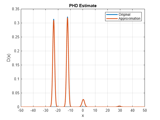
Visualize the PHD after pruning and merging to compare it with the original PHD. Notice that the PHD plot looks similar to the original plot and pruning, merging did not have a substantial impact on the PHD estimate.

Dapprox = arrayfun(@(e)calculatePHD(phd,e),x);
hold on;
h2 = plot(x, Dapprox, 'LineWidth',2);
legend('Original','Approximation');

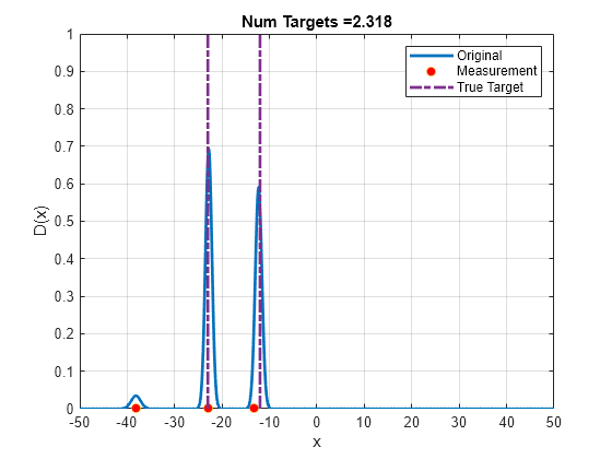
Run the PHD filter for few steps to see how the PHD function changes as more measurements are obtained. Notice that small peaks are observed at false alarms showing potential new objects, and the peaks at true target locations remain consistent. The sum of weights is close to 2, which shows that PHD filter estimates approximately 2 objects in the scene.

% Delete the approximation plot
delete(h2);

% For reproducible results
rng(0);

% Plot measurements on the X axes
hMeas = plot(0,0,'o','DisplayName','Measurement','MarkerFaceColor','r');

% Plot true targets as lines.
hTrue = plot([-23 -23 nan -12 -12],[0 10 nan 0 10],'-.','LineWidth',2,'DisplayName','True Target');
ylim([0 1]);

for i = 3:20
    Z = cell(3,1);
    Z{1} = objectDetection(i,-23 + sqrt(R)*randn,'MeasurementNoise',R);
    Z{2} = objectDetection(i,-12 + sqrt(R)*randn,'MeasurementNoise',R);
    Z{3} = objectDetection(i,50*(2*rand-1),'MeasurementNoise',R);
    
    % Predict PHD
    runPredictionIteration(phd, birthPHD, Ps);

    % Correct PHD
    runCorrectionIteration(phd, Z, Pd, Kc)
    
    % Merge and prune
    merge(phd, 5);
    prune(phd,phd.Weights < 0.001);
    
    D = arrayfun(@(e)calculatePHD(phd,e),x);
    h.YData = D;

    hMeas.XData = [Z{1}.Measurement Z{2}.Measurement Z{3}.Measurement];
    hMeas.YData = [0 0 0];
    title(['Num Targets =', num2str(sum(phd.Weights))]);
    drawnow;
end

Object State Estimation

In the previous sections, you learned how the PHD filter estimates the PHD in the state-space and how the peaks near true target locations become more prominent after updates. However, the goal of a multi-object tracking algorithm is to estimate the number of objects and their states and state uncertainties at each step. To estimate target states from the PHD, a variety of techniques can be used. The simplest technique is to calculate the expected number of targets (N) from the PHD function and extract the top N peaks from the PHD curve. Another popular method, which is facilitated by the Gaussian mixture approximation of the PHD, is by looking at the weights of each Gaussian component and extracting components with a weight higher than a pre-defined threshold. You can use the extractState method of the gmphd filter to get the state of components with a weight exceeding a certain threshold.

extractionThreshold = 0.3;
estimatedStates = extractState(phd,extractionThreshold)

estimatedStates=2×1 struct array with fields:
    State
    StateCovariance

Another key component of a multi-object tracker in some applications is to estimate the identity of the object across time. For the GM-PHD filter, this is typically done by assigning a label or an identity to each Gaussian component. During prediction and update steps, the label is propagated and preserved. A new label can be assigned to every peak extracted from the PHD as potential target. You can use the Labels property of the gmphd filter to assign these labels for maintenance. The filter preserves those labels during prediction and correction steps.

GM-PHD tracker

In the previous sections, you learned the different steps involved in running a PHD estimation and how to obtain the estimates about objects from the PHD. MATLAB also offers a multi-sensor GM-PHD tracker, trackerPHD, which performs the PHD recursion and extract the object states to produce outputs similar to data association based trackers such as trackerJPDA. In doing so, the trackerPHD uses the following assumptions.

For multi-sensor PHD update, the tracker performs an iterated correction, which means the tracker sequentially updates the PHD with every sensor. The order of the sensors is determined by the timestamp of the sensor observations. For two sensors sharing the same timestamp, the sensor order dictated by the SensorConfigurations property of the tracker is used.
The survival probability is modeled using a death rate, which defines $P_{s} = {(1 - DeathRate)}^{Δ T}$ . The death rate can be provided using the DeathRate property of the tracker.
Each sensor gets to define a predictive birth PHD and an adaptive birth PHD using the FilterInitializationFcn property of the SensorConfigurations. The sum of all components added by all the sensors is controlled by using the BirthRate property of the tracker. The tracker ensures that the sum of weights is equal to $BirthRate x Δ T$
Each sensor defines its own detection probability and clutter density using the DetectionProbability and ClutterDensity property of the trackingSensorConfiguration object.
For extracting labelled tracks from the PHD, the trackerPHD follows more customized pruning and merging schemes. When a peak is extracted as a potential track, it is provided a new label by the tracker. The extraction threshold is determined by the ExtractionThreshold property of the tracker. Tracker merges components using a merging threshold determined by MergingThreshold property of the tracker. While merging, components which are labelled are not allowed to merge with other labelled. At the end of multi-sensor PHD update, only 1 component per label is retained using the logic defined by LabelingThresholds property of the trackerPHD.

To use a different logic than the tracker, you can use the gmphd class and the recursion demonstrated in this example to build a customized logic.

Limitations

PHD filter is an attractive method for estimating the states of multiple objects as it accounts for data association uncertainty at a much cheaper cost. However, it has certain limitations. Most of these limitations arise due to approximating the multi-object pdf using a Poisson RFS. This greatly reduces the accuracy of the PHD filter in estimating the number of objects in the scene as the mean of a Poisson RFS is also its variance.

Summary

In this example, you learned how the PHD filter estimates the number of objects and their states in the environment. You learned how to use the gmphd filter and its methods to perform the PHD recursion and object state extraction.

function D = calculatePHD(phdObject, x)
D = 0;
m = phdObject.States;
P = phdObject.StateCovariances;
w = phdObject.Weights;
for i = 1:phdObject.NumComponents
    e = m(i) - x;
    gaussianPdf = 1/sqrt(det(2*pi*P(:,:,i)))*exp(-1/2*e'/P(:,:,i)*e);
    D = D + w(i)*gaussianPdf;
end
end

function s = logsumexp(x)
% This function calculates logsumexp(x). 
% logsumexp(x) = log(x(1) + x(2) + x(3) ..) given log(x(1)), log(x(2)) .. 
xmax = max(x);
xdiff = x - xmax;
s = xmax + log(sum(exp(xdiff)));
end

function Lij = calculateScaling(logqij, w, Pd, Kc)
% Our objective is to calculate
% Lij = Pd*qij/(Kc + sumOveri(Pd*qij*wi));
logPdqij = log(Pd) + logqij;

logPdqijwi = log(Pd) + logqij + log(w(:));

% Allocate sum of logPdqijwi over i.
logSumOverIPdqijwi = zeros(1,size(logqij,2));
for j = 1:size(logqij,2)
    logSumOverIPdqijwi(j) = logsumexp(logPdqijwi(:,j));
end

% Compute log(Kc + sumOveri(wi*Pd*qij));
den = zeros(1,size(logqij,2));
logKc = log(Kc);
for j = 1:size(logqij,2)
    den(j) = logsumexp([logKc;logSumOverIPdqijwi(j)]);
end

logLij = logPdqij - den;
Lij = exp(logLij);

end

function runPredictionIteration(phd, birthPHD, Ps)

% Predict existing components mean and covariances
predict(phd, 1);

% Scale by survival probability
scale(phd, Ps);

% Add birth PHD
append(phd, birthPHD);

end

function runCorrectionIteration(phd, Z, Pd, Kc)

% Undetected PHD
phdUndetected = clone(phd);
scale(phdUndetected, 1 - Pd);

% Inform PHD filter about detections at current step
phd.Detections = Z;

% detectionIndices
detectionIndices = eye(numel(Z),'logical'); 

% Calculate logqij
logqij = likelihood(phd, detectionIndices);

% Lij = Pd*qij/(Kc + Pd*sum(w*qij)). This calculation should be performed
% in logarithmic scale to avoid numerical issues.
Lij = calculateScaling(logqij, phd.Weights(:), Pd, Kc);

% Update the PHD filter. This is the detected PHD
correct(phd, detectionIndices, Lij);

% Add undetected PHD 
append(phd, phdUndetected);

end