Extended Object Tracking with Radar for Marine Surveillance

Open Script

This example shows how to generate a marine scenario, simulate radar detections from a marine surveillance radar, and configure a multi-target Probability Hypothesis Density (PHD) tracker to estimate the location and size of the simulated ships using the radar detections.

Marine Surveillance Scenario

Simulate a marine surveillance radar mounted at the top of a tower overlooking ships in a harbor. Simulation of the tower's location and the motion of the ships in the scenario is managed by trackingScenario.

% Create tracking scenario.
scenario = trackingScenario(StopTime = 30);

% Define unit conversions.
nmi2m = 1852;           % nautical miles to meters
hr2s = 3600;            % hours to seconds
kts2mps = nmi2m/hr2s;   % knots to meters per second

Marine Surveillance Radar

Add a marine surveillance radar to the tower. The radar is mounted 20 meters above sea level (ASL). The radar stares into the harbor, surveying a 30 degree azimuth sector. Common specifications for a marine surveillance radar are listed:

Sensitivity: 0 dBsm @ 5 km
Field of View: 30 deg azimuth, 10 deg elevation
Azimuth Resolution: 2 deg
Range Resolution: 5 m

Model the marine radar with the above specifications using the fusionRadarSensor.

% Create surveillance radar.
sensor = fusionRadarSensor(SensorIndex = 1, ...
    ScanMode = 'No scanning', ...
    MountingLocation = [0 0 -20], ...      % 20 meters (ASL)
    MountingAngles = [45 0 0], ...         % [yaw pitch roll] deg
    FieldOfView = [30 10], ...             % [az el] deg
    ReferenceRange = 5e3, ...              % m
    AzimuthResolution = 2, ...             % deg
    RangeResolution = 5, ...               % m
    HasINS = true,...                      % Report INS information
    TargetReportFormat = 'Detections',...  % Detections without clustering
    RangeLimits = [0 15e3], ...           % m
    DetectionCoordinates = 'Sensor spherical');

Add the tower to the scenario as a stationary platform with the radar mounted on top of it.

platform(scenario, Sensors = sensor);
tower = scenario.Platforms{1}

tower = 

  Platform with properties:

       PlatformID: 1
          ClassID: 0
         Position: [0 0 0]
      Orientation: [0 0 0]
       Dimensions: [1x1 struct]
             Mesh: [1x1 extendedObjectMesh]
       Trajectory: [1x1 kinematicTrajectory]
    PoseEstimator: [1x1 insSensor]
         Emitters: {}
          Sensors: {[1x1 fusionRadarSensor]}
       Signatures: {[1x1 rcsSignature]  [1x1 irSignature]  [1x1 tsSignature]}

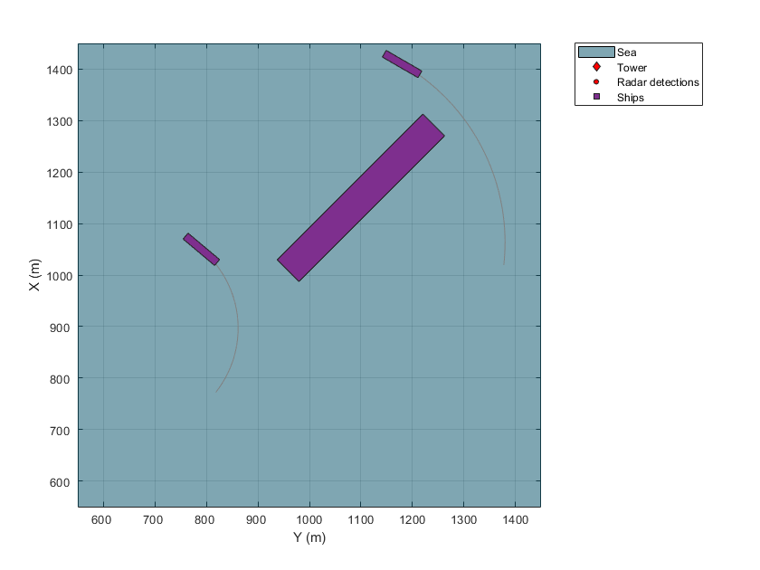
Add three ships in the harbor within the radar's surveillance sector. The two smaller ships are turning at 20 and 30 knots, the large ship is traveling at a constant heading at 10 knots.

% Define the dimensions for the two small ships.
dim = struct( ...
    Length = 80, ... % m
    Width = 15, ...  % m
    Height = 5, ...  % m
    OriginOffset = [0 0 5/2]); % [x y z] m

% Model the radar cross section (RCS) of the small ships as 30 dBsm.
rcs = rcsSignature('Pattern',30);

% Create a turning trajectory.
speed = 20;     % knots
initYaw = 130;  % deg
initPos = [1050 790 0];
radius = 200;   % m

initOrient = quaternion([initYaw 0 0], 'eulerd', 'ZYX', 'frame');
initVel = speed*kts2mps*rotatepoint(initOrient,[1 0 0])';
accBody = [0 (speed*kts2mps)^2/radius 0];
angVelBody = [0 0 speed*kts2mps/radius];
traj = kinematicTrajectory(Position = initPos, Velocity = initVel, Orientation = initOrient, ...
    AccelerationSource = 'Property', Acceleration = accBody, ...
    AngularVelocitySource = 'Property', AngularVelocity = angVelBody);

% Add the first small ship, traveling at 20 knots to the scenario. This is
% the closest ship to the radar tower.
platform(scenario, Dimensions = dim, Signatures = rcs, Trajectory = traj);

% Create the other small ship, traveling at 30 knots. This is the ship
% which is farthest from the radar tower.
speed = 30;     % knots
initYaw = 120;  % deg
initPos = [1410 1180 0];
radius = 400;   % m

initOrient = quaternion([initYaw 0 0],'eulerd','ZYX','frame');
initVel = speed*kts2mps*rotatepoint(initOrient,[1 0 0])';
accBody = [0 (speed*kts2mps)^2/radius 0];
angVelBody = [0 0 speed*kts2mps/radius];
traj = kinematicTrajectory(Position = initPos, Velocity = initVel, Orientation = initOrient, ...
    AccelerationSource = 'Property', Acceleration = accBody, ...
    AngularVelocitySource = 'Property', AngularVelocity = angVelBody);

platform(scenario, Dimensions = dim, Signatures = rcs, Trajectory = traj);

% Define the dimensions for the large ship.
dim = struct( ...
     Length = 400, ... % m
     Width = 60, ...   % m
     Height = 15, ...  % m
     OriginOffset = [0 0 15/2]); % [x y z] m

% Model the radar cross section (RCS) of the large ship as 75 dBsm.
rcs = rcsSignature(Pattern = 75);

% Create the large ship's trajectory, traveling at a constant heading at 10 knots.
speed = 10;     % knots
initYaw = -135; % degs
initPos = [1150 1100 0];

initOrient = quaternion([initYaw 0 0],'eulerd','ZYX','frame');
initVel = speed*kts2mps*rotatepoint(initOrient,[1 0 0])';
traj = kinematicTrajectory(Position = initPos, Velocity = initVel, Orientation = initOrient, ...
    AccelerationSource = 'Property', AngularVelocitySource = 'Property');

% Add the large ship to the scenario.
platform(scenario, Dimensions = dim, Signatures = rcs, Trajectory = traj);

% Create a display to show the true, measured, and tracked positions of the ships.
theaterDisplay = helperMarineSurveillanceDisplay(scenario, ...
     IsSea = true, DistanceUnits = 'm', ...
     XLim = 450*[-1 1]+1e3, YLim = 450*[-1 1]+1e3, ZLim = [-1000 10], ...
     Movie = 'MarineSurveillanceExample.gif');
slctTrkPos = zeros(3,7); slctTrkPos(1,1) = 1; slctTrkPos(2,3) = 1; slctTrkPos(3,6) = 1;
slctTrkVel = circshift(slctTrkPos,[0 1]);
theaterDisplay.TrackPositionSelector = slctTrkPos;
theaterDisplay.TrackVelocitySelector = slctTrkVel;
theaterDisplay();
snapnow(theaterDisplay);

Multi-Target GGIW-PHD Tracker

Create a trackerPHD to form tracks from the radar detections generated from the three ships in the harbor. The PHD tracker enables the estimation of the size of the ships by allowing multiple detections to be associated to a single object. This is important in situations such as marine surveillance where the size of the objects detected by the sensor is greater than the sensor's resolution, resulting in multiple detections generated along the surfaces of the ships.

The tracker uses the filterInitFcn supporting function to initialize a constant turn-rate Gamma Gaussian Inverse Wishart (GGIW) PHD filter. filterInitFcn adds birth components to the PHD-intensity at every time step. These birth components are added uniformly inside the field of view of the sensor. Their sizes and expected number of detections are specified using prior information about the types of ships expected in the harbor.

The tracker uses the gamma distribution of the GGIW-PHD components to estimate how many detections should be generated from an object. The tracker also calculates the detectability of each component in the density using the sensor's limits. Use trackingSensorConfiguration to model the sensor's configuration for trackerPHD.

%Create a trackingSensorConfiguration from the platform.
sensorConfig = trackingSensorConfiguration(tower, SensorTransformFcn = @ctmeas);

% Set FilterInitializationFcn
sensorConfig{1}.FilterInitializationFcn = @(varargin)filterInitFcn(varargin{:},sensorConfig{1}.SensorTransformParameters);

% Set DetectionProbablity for trackingSensorConfiguration
sensorConfig{1}.DetectionProbability = 0.99;

% % Noise covariance corresponding to a resolution cell of the radar.
resolutionNoise = diag((sensorConfig{1}.SensorResolution/2).^2);

% Create a PHD tracker using the trackingSensorConfiguration.
tracker = trackerPHD(SensorConfigurations = sensorConfig, ...
    HasSensorConfigurationsInput = true, ...
    PartitioningFcn = @(x)partitionDetections(x,2,6), ...
    MergingThreshold=75,...
    ExtractionThreshold = 0.75,...
    DeletionThreshold = 1e-6,...
    BirthRate = 1e-5);

Simulate and Track Ships

The following loop advances the positions of the ships until the end of the scenario. For each step forward in the scenario, the tracker is updated with the detections from the ships in the radar's field of view.

% Initialize scenario and tracker.
restart(scenario);
reset(tracker);

% Set simulation to advance at the update rate of the radar.
scenario.UpdateRate = sensor.UpdateRate;

% Set random seed for repeatable results.
rng(1,'twister');

% Run simulation.
snapTimes = [2 7 scenario.StopTime]; % seconds
while advance(scenario)
    % Get current simulation time.
    time = scenario.SimulationTime;

    % Generate detections from the tower's radar.
    [dets,~,config] = detect(tower,time);

    % Update measurement noise of detections to match radar's resolution.
    dets = updateMeasurementNoise(dets,resolutionNoise);

    % Update tracker.
    tracks = tracker(dets,config,time);

    % Update display with current beam position, detections, and track positions.
    theaterDisplay(dets,config,tracks);

    % Take snapshot.
    snapFigure(theaterDisplay,any(time==snapTimes));
end
writeMovie(theaterDisplay);

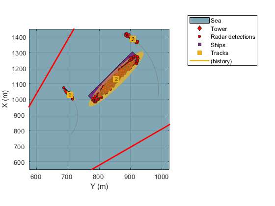
The following figure shows the radar detections, shown as red dots, and the estimated track locations, shown as yellow squares annotated with the track ID, and the estimated tracked object's extent, shown as a yellow ellipse. The radar tower is located at the origin, (0,0), which is not shown in the figure. The radar's field of view is indicated by the two red lines crossing the top and bottom of the figure. All of the ships lie within the radar's field of view, and because the size of the ships is much larger than the radar's range and azimuth resolution, multiple detections are made along the faces of the ships visible to the radar.

showSnapshot(theaterDisplay,1)

Because the ships are modeled as extended objects and not point targets, detections of a ship can be occluded by the presence of another ship between the ship and the radar. This is shown in the following figure. In this case, the smaller ship at the top of the figure is not detected by the radar. The radar's line of sight is occluded by both the other small ship at the bottom of the figure and the large ship in the center. The tracker maintains an estimate of the occluded ship and associates detections in the following steps to the track without ever dropping the track.

showSnapshot(theaterDisplay,2)
axis([1250 1450 1150 1350]); view([-90 90]);

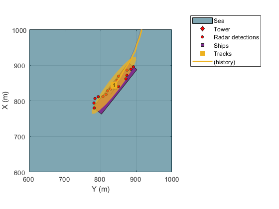
The following figure shows the PHD estimate of the smaller ship located closest to the radar in the scenario. You can verify the PHD estimate of the ship's location lies near the center of the ship and the estimated size is reasonably close to the actual size of the ship, indicated by the overlap of the track's ellipse with the ship.

showSnapshot(theaterDisplay,3)
axis([650 850 700 900]); view([-90 90]);

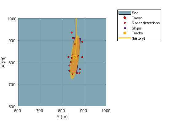
The next figure also shows that the PHD tracker estimated both the location, size, and heading of the other small ship in the scenario. This is the ship that was previously occluded by the other two ships. Despite the occlusion, the estimated location, size, and orientation closely matches the ship.

showSnapshot(theaterDisplay,3)
axis([900 1100 1250 1450]); view([-90 90]);

The track states of the 3 ships report the estimated size of each ship using a 3D positional covariance matrix. Take the eigen decomposition of the covariance matrices to compute the estimated length, width, and height for each of the ships.

numTrks = numel(tracks);
TrackID = [tracks.TrackID]';
Length = zeros(numTrks,1);
Width = zeros(numTrks,1);
Height = zeros(numTrks,1);
for iTrk = 1:numTrks
    ext = tracks(iTrk).Extent;
    [Q,D] = eig(ext);
    d = 2*sqrt(diag(D));
    iDims = 1:3;

    up = [0 0 -1];
    [~,iUp] = max(abs(up*Q));
    Height(iTrk) = d(iDims(iUp));
    iDims(iUp) = [];

    Length(iTrk) = max(d(iDims));
    Width(iTrk) = min(d(iDims));
end

% Display a table of the estimated dimensions of the ships.
dims = table(TrackID,Length,Width,Height)

dims =

  3x4 table

    TrackID    Length    Width     Height
    _______    ______    ______    ______

       1       100.79    17.547    16.244
       2       473.51    52.247    8.8432
       3       99.688    18.585    17.443

Recall that the true dimensions of the ships are given by:

Large Ship

Length: 400 m
Width: 60 m
Height: 15 m

Small Ship

Length: 80 m
Width: 15 m
Height: 5 m

The tracker is able to differentiate between the size of the large and smaller ships by estimating the shape of each ship as an ellipse. In the simulation, the true shape of each ship is modeled using a cuboid. This mismatch between the shape assumption made by the tracker and the true shapes of the modeled ships results in overestimates the length and width of the ships. The radar is a 2D sensor, only measuring range and azimuth, so the height of each ship is not observable. This results in inaccurate height estimates reported by the tracker.

Summary

This example shows how to generate a marine scenario, simulate radar detections from a marine surveillance radar, and configure a multi-target PHD tracker to track the simulated ships using the radar detections. In this example, you learned how to model extended objects in a scenario, generating multiple detections from these objects. You also learned how to use a multi-target PHD tracker to process the information provided by the multiple detections to estimate not only the location but also the size of the tracked objects.

Supporting Functions

updateMeasurementNoise

Sets the measurement noise of the detections based on the specified noise covariance.

function dets = updateMeasurementNoise(dets,noise)
    for iDet = 1:numel(dets)
        dets{iDet}.MeasurementNoise(:) = noise(:);
    end
end

filterInitFcn

Modifies the filter returned by initctggiwphd to match the velocities and expected number of detections for the ships being tracked.

function phd = filterInitFcn(measParam,varargin)
% This function uses the predictive birth density only to simulate birth in
% the scenario.

if nargin == 1 % Set predictive birth uniformly inside the FOV.
    phdDefault = initctggiwphd;
    % 1. Create uniformly distributed states using Azimuth and Range.
    az = 0; % All components at azimuth.
    ranges = linspace(1000,10000,5); % 5 components for range
    [Az,R] = meshgrid(az,ranges);

    % create a PHD filter to allocate memory.
    phd = ggiwphd(zeros(7,numel(Az)),repmat(eye(7),[1 1 numel(Az)]),...
         ScaleMatrices = repmat(eye(3),[1 1 numel(Az)]),...
         StateTransitionFcn = @constturn, StateTransitionJacobianFcn = @constturnjac,...
         MeasurementFcn = @ctmeas, MeasurementJacobianFcn = @ctmeasjac,...
         PositionIndex = [1 3 6], ExtentRotationFcn = phdDefault.ExtentRotationFcn,...
         HasAdditiveProcessNoise = false, ProcessNoise = 2*eye(4),...
         TemporalDecay = 1e3, GammaForgettingFactors = 1.1*ones(1,numel(Az)),...
         MaxNumComponents = 10000);

    for i = 1:numel(Az)
        [sensorX,sensorY,sensorZ] = sph2cart(deg2rad(Az(i)),0,R(i));
        globalPos = measParam(1).Orientation'*[sensorX;sensorY;sensorZ] + measParam(1).OriginPosition(:);
        phd.States([1 3 6],i) = globalPos;
        phd.StateCovariances([1 3 6],[1 3 6],i) = diag([1e5 1e5 1000]); % Cover gaps between components using position covariance
    end

    % 2. You have described the "kinematic" states of each of the ships
    % inside the field of view. Next, add information about their sizes and
    % expected number of detections.
    %
    % It is expected that there are 2 types of ships in the sea, small and
    % large. You create components for each size.
    phdSmall = phd;

    % Clone the PHD filter for large ships.
    phdLarge = clone(phd);

    % Set initial number of components.
    numComps = phdSmall.NumComponents;

    % For small ships, the expected size is about 100 meters in length and
    % 20 meters in width. As the orientation is unknown, we will create 4
    % orientations for each size. First, you must add components to the
    % density at same states. This can be done by simply appending it
    % Setup values for small boats
    append(phdSmall,phdSmall);
    append(phdSmall,phdSmall);

    % Degrees of freedom for defining shape. A large number represents
    % higher certainty in dimensions.
    dof = 1000;

    % Covariance in vx, vy and omega.
    smallStateCov = diag([300 300 50]);

    % Scale matrix for small boats
    smallShape = (dof - 4)*diag([100/2 20/2 10].^2); % l, w and h

    % Create 4 orientations at 45 degrees from each other.
    for i = 1:4
        thisIndex = (i-1)*numComps + (1:numComps);
        R = rotmat(quaternion([45*(i-1) 0 0],'eulerd','ZYX','frame'),'frame');
        phdSmall.ScaleMatrices(:,:,thisIndex) = repmat(R*smallShape*R',[1 1 numComps]);
        phdSmall.StateCovariances([2 4 5],[2 4 5],thisIndex) = repmat(R*smallStateCov*R',[1 1 numComps]);
        phdSmall.StateCovariances([6 7],[6 7],thisIndex) = repmat(diag([100 100]),[1 1 numComps]);
    end

    % Small ships generate approximately 10-20 detections.
    expNumDets = 15;
    uncertainty = 5^2;
    phdSmall.Rates(:) = expNumDets/uncertainty;
    phdSmall.Shapes(:) = expNumDets^2/uncertainty;
    phdSmall.DegreesOfFreedom(:) = dof;

    % Follow similar process for large ships.
    append(phdLarge,phdLarge);
    append(phdLarge,phdLarge);
    largeStateCov = diag([100 5 10]);
    largeShape = (dof - 4)*diag([500/2 100/2 10].^2);
    for i = 1:4
        thisIndex = (i-1)*numComps + (1:numComps);
        R = rotmat(quaternion([45*(i-1) 0 0],'eulerd','ZYX','frame'),'frame');
        phdLarge.ScaleMatrices(:,:,thisIndex) = repmat(R*largeShape*R',[1 1 numComps]);
        phdLarge.StateCovariances([2 4 5],[2 4 5],thisIndex) = repmat(R*largeStateCov*R',[1 1 numComps]);
        phdLarge.StateCovariances([6 7],[6 7],thisIndex) = repmat(diag([100 100]),[1 1 numComps]);
    end

    % Generate approximately 100-200 detections.
    expNumDets = 150;
    uncertainty = 50^2;
    phdLarge.Rates(:) = expNumDets/uncertainty;
    phdLarge.Shapes(:) = expNumDets^2/uncertainty;
    phdLarge.DegreesOfFreedom(:) = dof;

    % Add large ships to small ships to create total density. This density
    % is added to the total density every step.
    phd = phdSmall;
    append(phd,phdLarge);
end

% When called with detection input i.e. the adaptive birth density, do not
% add any new components.
if nargin > 1
    % This creates 0 components in the density.
    phd = initctggiwphd;
end
end