Passive Ranging Using a Single Maneuvering Sensor

Open Script

This example illustrates how to track targets using passive angle-only measurements from a single sensor. Passive angle-only measurements contain azimuth and elevation of a target with respect to the sensor. The absence of range measurements makes the problem challenging as the targets to be tracked are fully observable only under certain conditions.

In this example, you learn about some possible solutions to this problem by using a passive infrared sensor mounted on a maneuvering platform.

Introduction

The absence of range measurements from a target implies incomplete observability of the target state. The following figure depicts that angle-only measurements obtained by an observer traveling at a constant velocity results in multiple possible trajectories of a (presumed constant velocity) target.

Theoretical results imply that the target state is unobservable until the following conditions are met [1].

The sensor must out-maneuver the target i.e. the sensor motion must be at least 1 order higher than the target. For example, if a target is traveling at constant velocity, the observer must have at least a constant acceleration.
The component of sensor maneuver perpendicular to line of sight must be non-zero.

Define Scenario

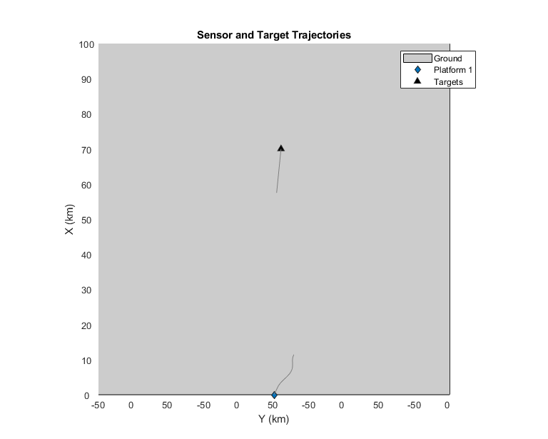
A helper function helperCreatePassiveRangingScenario is used to define a single infrared sensor mounted on a platform. The sensing platform, often termed as ownship, travels at constant velocity in the beginning and then performs a maneuver to observe the range of the target. The target is assumed to be non-maneuvering and travels at a constant velocity in the scenario.

% Setup
[scene,ownship,theaterDisplay] = helperCreatePassiveRangingScenario;
showScenario(theaterDisplay);

Track Using an EKF in Cartesian Coordinates

The problem of tracking a target using angle-only measurements can be formulated using an extended Kalman filter with a non-linear measurement model in Cartesian coordinates. In this section, a constant velocity trackingEKF, describing the state in global Cartesian coordinates is used to track the target.

% Set random seed for reproducible results
rng(50);

% Create a |trackerGNN| to track the targets using the
% FilterInitializationFcn as @initCartesianEKF.
tracker = trackerGNN('FilterInitializationFcn',@initCartesianEKF,...
    'AssignmentThreshold',50,...
    'MaxNumTracks',5);

[tem, tam] = helperPassiveRangingErrorMetrics(ownship,false);

theaterDisplay.ErrorMetrics = tem;

tracks = [];

% Advance scenario, simulate detections and track
while advance(scene)
    % Get time information from tracking scenario.
    truths = platformPoses(scene);
    time = scene.SimulationTime;

    % Generate detections from the ownship
    detections = detect(ownship,time);

    % Pass detections to tracker
    if ~isempty(detections)
        tracks = tracker(detections,time);
    elseif isLocked(tracker)
        tracks = predictTracksToTime(tracker,'confirmed',time);
    end
    % Update error and assignment metrics
    tam(tracks,truths);
    [trackIDs, truthIDs] = currentAssignment(tam);
    tem(tracks,trackIDs,truths,truthIDs);

    % Update display
    theaterDisplay(tracks,detections,tracker);
end

The track is initialized using a high covariance in range to account for the missing measurement. Notice the covariance in range of the track just after initialization in the theater plot. As angular estimates are fairly accurate, the target uncertainty is described by a thin covariance ellipse.

showGrabs(theaterDisplay,1);

The following figure shows the filter performance after the sensor starts maneuvering in the scenario. The range and range-rate estimate plots are created using errorbar and show the $\sigma$ (standard deviation) bounds of the track's estimate.

showGrabs(theaterDisplay,2);

Stability of EKF in Cartesian Coordinates

Tracking in Cartesian coordinates using an extended Kalman filter is appealing due to the ease of problem formulation. The state dynamics are represented by a set of linear equations and the non-linearities are embedded using two (relatively) simple equations for azimuth and elevation.

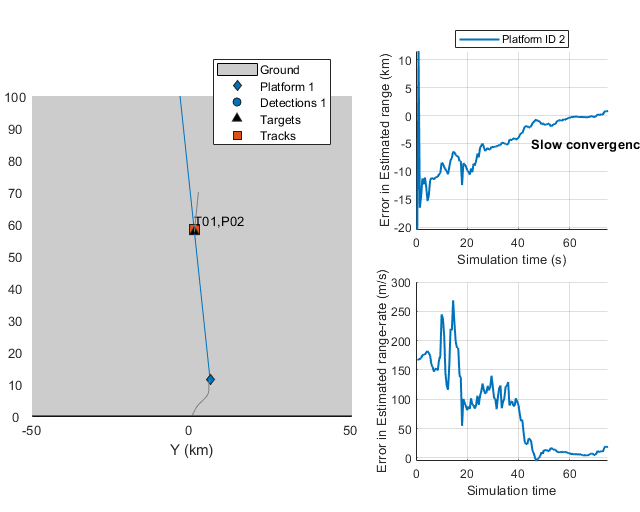
That said, the behavior of the extended Kalman filter is shown to be erratic and can often be unstable. This is because the states (position and velocity) and unobservable range are highly coupled. When range is unobservable, i.e., during the constant velocity phase of the sensing platform motion, the filter "falsely" estimates the range of the target depending on the history of measurement and associated noise values. This can result in a premature collapse of the covariance ellipse, which can cause the filter to take a very long time to converge (or even diverge) [2] even after sufficient observability conditions are met.

Use a different random seed to observe premature convergence of an extended Kalman filter in Cartesian coordinates.

% set random seed
rng(2015);

% Reset the theaterDisplay to capture snapshots with new scenario.
release(theaterDisplay);
theaterDisplay.GrabFigureFcn = @(fig,scene)helperGrabPassiveRangingDisplay(fig,scene,'CartEKF2');
helperRunPassiveRangingSimulation(scene,theaterDisplay,@initCartesianEKF);

After 2 seconds, the covariance in the range has already collapsed, making the filter falsely confident about its estimate of the range. Notice that target lies outside the covariance ellipse of the track's state and so does the zero-error line in the range estimation plot.

showGrabs(theaterDisplay,3);

Because the filter remains confident about it estimate of the range, it takes much longer to converge closer to actual range values.

showGrabs(theaterDisplay,4);

Track Using an EKF in Modified Spherical Coordinates (MSC-EKF)

The modified spherical coordinates (MSC) present a stable coordinate system for tracking using angle-only measurements. By decoupling the state into observable and unobservable parts, the filter overcomes the limitations imposed by the EKF in Cartesian coordinates. The state in modified spherical coordinates is defined in a relative manner i.e. [target - observer] and hence an input from the observer is required to predict the state in future. This can be seen in the following equations where higher order terms refer to observer motion not captured by a constant velocity model.

$x = x_{t} - x_{o}$

$\dot{x} = \dot{x_{t}} - \dot{x_{o}}$

$\dot{x} = Ax_{t} - (Ax_{0} + \mathcal{O}(t^{2}) + \mathcal{O}(t^{3}) + ..)$

$\dot{x} = A(x_{t} - x_{0}) + \mbox{ higher} \mbox{ order} \mbox{ terms}$

% Set the same random seed to compare with the same detections
rng(2015);

% restart the scene
restart(scene);
release(theaterDisplay);
theaterDisplay.GrabFigureFcn = @(fig,scene)helperGrabPassiveRangingDisplay(fig,scene,'MSCEKF');

[tem, tam] = helperPassiveRangingErrorMetrics(ownship,true);
theaterDisplay.ErrorMetrics = tem;

% Create a tracker using |trackerGNN| and MSC-EKF filter initialization.
tracker = trackerGNN('FilterInitializationFcn',@initMSCEKF,...
    'AssignmentThreshold',50);

% The tracks carry a state which is non-linearly dependent on position.
% Inform the theaterDisplay that tracks have non-linear state and position
% can be extracted using a function_handle.
theaterDisplay.HasNonLinearState = true;
theaterDisplay.NonLinearTrackPositionFcn = @getTrackPositionsMSC;

% Initialization for MSC-EKF.
prevPose = pose(ownship,'true');
lastCorrectionTime = 0;
allTracks = [];

% Advance scenario, simulate detections and track
while advance(scene)

    time = scene.SimulationTime;
    truths = platformPoses(scene);

    % Generate detections from ownship
    detections = detect(ownship,time);

    % Update the input from the ownship i.e. it's maneuver since last
    % correction time.
    currentPose = pose(ownship,'true');
    dT = time - lastCorrectionTime;
    observerManeuver = calculateManeuver(currentPose,prevPose,dT);

    for i = 1:numel(allTracks)
        % Set the ObserverInput property using |setTrackFilterProperties|
        % function of the tracker
        setTrackFilterProperties(tracker,allTracks(i).TrackID,'ObserverInput',observerManeuver);
    end

    % Pass detections to tracker
    if ~isempty(detections)
        lastCorrectionTime = time;
        % Store the previous pose to calculate maneuver
        prevPose = currentPose;
        [tracks,~,allTracks] = tracker(detections,time);
    elseif isLocked(tracker)
        tracks = predictTracksToTime(tracker,'confirmed',time);
    end

    % Update error and assignment metrics
    tam(tracks,truths);
    [trackIDs, truthIDs] = currentAssignment(tam);
    tem(tracks,trackIDs,truths,truthIDs);

    % Update display
    theaterDisplay.NonLinearStateInput = currentPose.Position(:);
    theaterDisplay(detections,tracks,tracker);
end

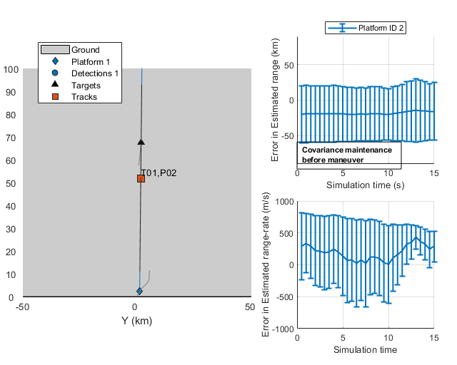
The MSC-EKF tries to maintain the covariance in range till the sensor has not made a maneuver. This is essentially due to decoupled observable and unobservable parts in the state.

showGrabs(theaterDisplay,5);

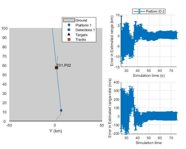
The filter converges closer to true values faster than the EKF in Cartesian coordinates and the $\sigma$ bounds provide a true, unbiased estimate of the error.

showGrabs(theaterDisplay,6);

Track Using a Range-Parameterized MSC-EKF

The MSC-EKF approach uses linearization techniques to project covariances in the prediction step. The covariance in range at initialization is typically high and the state transition dynamics is highly non-linear, which can cause issues with filter convergence.

This section demonstrates the use of a Gaussian-sum filter, trackingGSF, to describe the state with a bank of filters, each initialized at different range assumptions. This technique is commonly termed as range-parameterization [3].

% Set random seed
rng(2015);

% restart the scene
restart(scene);
release(theaterDisplay);
theaterDisplay.GrabFigureFcn = @(fig,scene)helperGrabPassiveRangingDisplay(fig,scene,'MSCRPEKF');

% Create error and assignment metrics.
[tem, tam] = helperPassiveRangingErrorMetrics(ownship,true);
theaterDisplay.ErrorMetrics = tem;

% Create a tracker using |trackerGNN| and range-parameterized MSC-EKF
% filter initialization.
tracker = trackerGNN('FilterInitializationFcn',@initMSCRPEKF,...
    'AssignmentThreshold',50);

theaterDisplay.HasNonLinearState = true;
theaterDisplay.NonLinearTrackPositionFcn = @getTrackPositionsMSC;

% Initialization for MSC-RPEKF
prevPose = pose(ownship,'true');
lastCorrectionTime = 0;
allTracks = [];

% Advance scenario, simulate detections and track
while advance(scene)

    time = scene.SimulationTime;
    truths = platformPoses(scene);

    % Generate detections from ownship
    detections = detect(ownship,time);

    % Update the input from the ownship i.e. it's maneuver since last
    % correction time.
    currentPose = pose(ownship,'true');
    dT = time - lastCorrectionTime;
    observerManeuver = calculateManeuver(currentPose,prevPose,dT);

    % Get each filter from the trackingGSF property TrackingFilters using
    % the |getTrackFilterProperties| function of the tracker.
    for i = 1:numel(allTracks)
        trackingFilters = getTrackFilterProperties(tracker,allTracks(i).TrackID,'TrackingFilters');
        % Set the ObserverInput for each tracking filter
        for m = 1:numel(trackingFilters{1})
            trackingFilters{1}{m}.ObserverInput = observerManeuver;
        end
    end

    % Pass detections to tracker
    if ~isempty(detections)
        lastCorrectionTime = time;
        % Store the previous pose to calculate maneuver
        prevPose = currentPose;
        [tracks,~,allTracks] = tracker(detections,time);
    elseif isLocked(tracker)
        tracks = predictTracksToTime(tracker,'confirmed',time);
    end

    % Update error and assignment metrics
    tam(tracks,truths);
    [trackIDs, truthIDs] = currentAssignment(tam);
    tem(tracks,trackIDs,truths,truthIDs);

    % Update display
    theaterDisplay.NonLinearStateInput = currentPose.Position(:);
    theaterDisplay(detections,tracks,tracker);
end

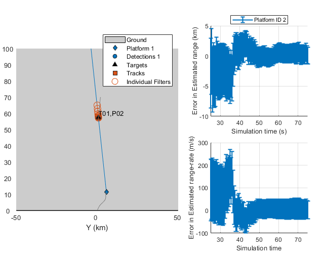
The following figures show the range-parameterized filter after track is initialized and the tracking performance of the filter. The range-parameterization process allows each filter to carry a relatively small covariance in range and hence is less susceptible to linearization issues. The time-to-converge for range-parametrized filter in this scenario is similar to the MSC-EKF. However, the filter demonstrated less transient behavior as the sensor moves into the second major maneuvering phase of the trajectory, i.e., 35 to 40 seconds into simulation. Notice, the MSC-EKF range estimation plot above, which produced an error of 10+ km in range. The estimation error was about 5 km for the range-parametrized filter.

showGrabs(theaterDisplay,[7 8]);

Close displays

showGrabs(theaterDisplay,[]);

Multi-Target Scenarios

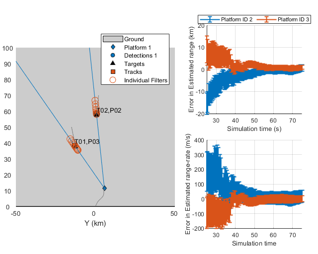
The demonstrated approach using MSC-EKF and range-parameterized MSC-EKF is applicable for more than 1 target. To observe each target, the sensor must out-maneuver each one of them. As filters like MSC-EKF can maintain range-covariance during non-maneuvering stages, each track's estimate should converge closer to the targets as the sensor makes maneuvers with respect to them.

MSC-EKF

% Set random seed
rng(2015);

% Create a two-target scenario and theater display.
[sceneTwo,~,theaterDisplayTwo] = helperCreatePassiveRangingScenario(2);

% Use the helper function to run the simulation using @initMSCEKF.
helperRunPassiveRangingSimulation(sceneTwo,theaterDisplayTwo,@initMSCEKF);

% Show results
showGrabs(theaterDisplayTwo,1);

Range-parameterized MSC-EKF

% Set random seed
rng(2015);
release(theaterDisplayTwo);

% Run the simulation using range-parameterized MSC-EKF
helperRunPassiveRangingSimulation(sceneTwo,theaterDisplayTwo,@initMSCRPEKF);

% Show results
showGrabs(theaterDisplayTwo,2);

Summary

This example illustrates the challenges associated with single-sensor angle-only tracking problem and demonstrates how to use different tracking algorithms to estimate target's range and range-rate. You learned how to use initcvekf, initcvmscekf and trackingGSF to define customized Cartesian-EKF, MSC-EKF and range-parameterized MSC-EKF for passive ranging. You also learned how to use the defined filters with a GNN tracker, trackerGNN.

Supporting Functions

Filter initialization Functions

The following section lists all the FilterInitializationFcn used for the trackerGNN object in this Example.

initCartesianEKF Initialize trackingEKF from an angle-only detection

function filter = initCartesianEKF(detection)

% Create a full detection with high covariance in range estimate.
rangeEstimate = 5e4;
rangeCov = 16e8;
fullDetection = detection;
fullDetection.Measurement = [fullDetection.Measurement;rangeEstimate];
fullDetection.MeasurementNoise = blkdiag(fullDetection.MeasurementNoise,rangeCov);

% Update the MeasurementParameters to include range.
fullDetection.MeasurementParameters(1).HasRange = true;

% Use the initcvekf function to initialize a trackingEKF using the
% fullDetection.
fullFilter = initcvekf(fullDetection);

% |initcvekf| defines the StateCovariance in velocity with 100. This
% defines a standard deviation uncertainty in velocity as 10 m/s. Scale
% the velocity covariance with 400 i.e. an equivalent velocity standard
% deviation of 200 m/s
velCov = fullFilter.StateCovariance(2:2:end,2:2:end);
fullFilter.StateCovariance(2:2:end,2:2:end) = 400*velCov;

% fullFilter can only be corrected with [az el r] measurements.
% Create a |trackingEKF| using the State and StateCovariance from
% fullFilter.
filter = trackingEKF(@constvel,@cvmeas,fullFilter.State,...
    'StateCovariance',fullFilter.StateCovariance,...
    'StateTransitionJacobianFcn',@constveljac,...
    'MeasurementJacobianFcn',@cvmeasjac,...
    'HasAdditiveProcessNoise',false);

% Unit standard deviation acceleration noise
filter.ProcessNoise = eye(3);

end

initMSCEKF Initialize a MSC-EKF from an angle-only detection

function filter = initMSCEKF(detection)
% Use the second input of the |initcvmscekf| function to provide an
% estimate of range and standard deviation in range.
rangeEstimate = 5e4;
rangeSigma = 4e4;
filter = initcvmscekf(detection,[rangeEstimate,rangeSigma]);
% The initcvmscekf assumes a velocity standard deviation of 10 m/s, which
% is linearly transformed into azimuth rate, elevation rate and vr/r.
% Scale the velocity covariance by 400 to specify that target can move 20
% times faster.
filter.StateCovariance(2:2:end,2:2:end) = 400*filter.StateCovariance(2:2:end,2:2:end);
filter.ProcessNoise = eye(3);
end

initMSCRPEKF Initialize a range-parameterized MSC-EKF from an angle-only detection

function filter = initMSCRPEKF(detection)
% A range-parameterized MSC-EKF can be defined using a Gaussian-sum filter
% (trackingGSF) containing multiple |trackingMSCEKF| as TrackingFilters.

% Range-parametrization constants
rMin = 3e4;
rMax = 8e4;
numFilters = 10;
rho = (rMax/rMin)^(1/numFilters);
Cr = 2*(rho - 1)/(rho + 1)/sqrt(12);
indFilters = cell(numFilters,1);
for i = 1:numFilters
    range = rMin/2*(rho^i + rho^(i-1));
    rangeSigma = Cr*range;
    % Use initcvmscekf function to create a trackingMSCEKF with provided
    % range and rangeSigma.
    indFilters{i} = initcvmscekf(detection,[range rangeSigma]);
    % Update the velocity covariance of each filter.
    indFilters{i}.StateCovariance(2:2:end,2:2:end) = 400*indFilters{i}.StateCovariance(2:2:end,2:2:end);
end
filter = trackingGSF(indFilters);

end

Utility functions calculateManeuver

function maneuver = calculateManeuver(currentPose,prevPose,dT)
% Calculate maneuver i.e. 1st order+ motion of the observer. This is
% typically obtained using sensors operating at much higher rate.
v = prevPose.Velocity;
prevPos = prevPose.Position;
prevVel = prevPose.Velocity;
currentPos = currentPose.Position;
currentVel = currentPose.Velocity;

% position change apart from constant velocity motion
deltaP = currentPos - prevPos - v*dT;
% Velocity change
deltaV = currentVel - prevVel;

maneuver = zeros(6,1);
maneuver(1:2:end) = deltaP;
maneuver(2:2:end) = deltaV;
end

getTrackPositionsMSC

function [pos,cov] = getTrackPositionsMSC(tracks,observerPosition)

if isstruct(tracks) || isa(tracks,'objectTrack')
    % Track struct
    state = [tracks.State];
    stateCov = cat(3,tracks.StateCovariance);
elseif isa(tracks,'trackingMSCEKF')
    % Tracking Filter
    state = tracks.State;
    stateCov = tracks.StateCovariance;
end

% Get relative position using measurement function.
relPos = cvmeasmsc(state,'rectangular');

% Add observer position
pos = relPos + observerPosition;
pos = pos';

if nargout > 1
    cov = zeros(3,3,numel(tracks));

    for i = 1:numel(tracks)
        % Jacobian of position measurement
        jac = cvmeasmscjac(state(:,i),'rectangular');
        cov(:,:,i) = jac*stateCov(:,:,i)*jac';
    end
end

end

References

[1] Fogel, Eli, and Motti Gavish. "Nth-order dynamics target observability from angle measurements." IEEE Transactions on Aerospace and Electronic Systems 24.3 (1988): 305-308.

[2] Aidala, Vincent, and Sherry Hammel. "Utilization of modified polar coordinates for bearings-only tracking." IEEE Transactions on Automatic Control 28.3 (1983): 283-294.

[3] Peach, N. "Bearings-only tracking using a set of range-parameterised extended Kalman filters." IEE Proceedings-Control Theory and Applications 142.1 (1995): 73-80.