Smooth Trajectory Estimation of `trackingIMM` Filter

Since R2021b

This example shows how to smooth state estimates of a target using the smooth object function. Smoothing is a technique to refine previous state estimates using the up-to-date measurements and the state estimate information. In this example, you will learn how to improve previously corrected estimates from an Interacting Multi-Model (IMM) filter by running a backward recursion, which produces smoothed and more accurate state estimates. In the first section, you implement a smooth algorithm to smooth the trajectory of a turning car. In the remainder of this example, you perform smoothing on several highly maneuvering aircraft trajectories, taken from the Benchmark Trajectories for Multi-Object Tracking example.

Fixed Interval Smoothing to Track Turning Car

In this section, you smooth the trajectory estimate of a turning car. First, you use the helperGenerateCarMeasurements function to generate the position measurements of the car and the corresponding truth.

rng(2021); % For repeatable results

% Generate measurements for a car taking a turn
[measPositionCar, trueStateCar, timeCar] = helperGenerateCarMeasurements();

% Define the initial detection in the format of objectDetection
detection = objectDetection(0, [0;0;0], 'MeasurementNoise', eye(3,3));

Using the initekfimm initialization function, you create an IMM filter based on the constant velocity, constant acceleration, and constant turn motion models. To setup the filter for backward smoothing, you set the EnableSmoothing property of the filter to true. Since you want to perform fixed interval smoothing (offline smoothing) on the state estimates, which utilizes all corrected and predicted steps, you set the MaxNumSmoothingSteps property to the number of measurement steps.

defaultIMMCar = initekfimm(detection);
% Enable Smoothing
defaultIMMCar.EnableSmoothing = true;
defaultIMMCar.MaxNumSmoothingSteps = size(measPositionCar,1);
% Initilaize IMM
positionSelector = [1 0 0 0 0 0;0 0 1 0 0 0;0 0 0 0 1 0]; % Select position from state
initialState = positionSelector' * measPositionCar(1,:)';
initialCovariance = diag([1,1e4,1,1e4,1,1e4]);
initialize(defaultIMMCar, initialState, initialCovariance);

To obtain the forward estimates of the car, you run the filter by iteratively predicting and correcting the state estimates.

% Initialize the corrected states
numSteps = numel(timeCar);
correctState = zeros(6,numSteps);
correctStateCovariance = zeros(6,6,numSteps);
correcState(:,1) = defaultIMMCar.State;
correctStateCovariance(:,:,1) = defaultIMMCar.StateCovariance;

% Forward tracking with prediction and correction
for i = 2:numSteps
    dt = timeCar(i) - timeCar(i-1);
    predict(defaultIMMCar, dt);
    [correctState(:,i), correctStateCovariance(:,:,i)] = correct(defaultIMMCar, measPositionCar(i,:));
end

To perform the smoothing, simply call the smooth object function of the filter. The function returns the smoothed states, state covariance, and model probabilities.

[smoothState, smoothStateCovariance, modelProbabilities] = smooth(defaultIMMCar);

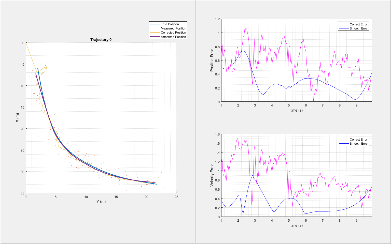
Next, use the helperTrajectoryViewer function to visualize the smooth results and the RMS errors. The results show that using offline smoothing of an IMM filter enables you to reduce the errors in estimates.

trajNum = 0;
helperTrajectoryViewer(trajNum,timeCar,correctState, smoothState, trueStateCar, measPositionCar);

Smooth Highly Maneuvering Aircraft Trajectories with Default IMM Configuration

In this section, you smooth the trajectories of six highly maneuvering aircraft. The trajectories used in this section are the same as those in the Benchmark Trajectories for Multi-Object Tracking example. In the example, the aircraft acceleration changes as much as 35 $m / s^{2}$ during some of the maneuvers. You use the helperGenerateAircraftTrajMeasurements function to generate the measurement data and truth.

[measPosition, trueState, time] = helperGenerateAircraftTrajMeasurements;

Configure an IMM filter similar as the previous section.

% Define initial detection
detection = objectDetection(0, [0;0;0], 'MeasurementNoise', eye(3,3));

defaultIMMAircraft = initekfimm(detection);
% Enable Smoothing
defaultIMMAircraft.EnableSmoothing = true;
defaultIMMAircraft.MaxNumSmoothingSteps = size(measPosition,1);

Using the helperGenerateSmoothData function, you run the created IMM filter, obtain the corrected state estimates, and generate the smoothed state estimates for the first trajectory.

% Only estimate the first trajectory
trajNum = 1;

% Extract measurement data
measPosTraj = measPosition(:,:,trajNum);

% Estimate and smooth the trajectory using the helperGenerateSmoothData function
[correctState, correctStateCovariance, smoothState, smoothStateCovariance] = helperGenerateSmoothData(defaultIMMAircraft,measPosTraj,time);

Visualize the forward estimation and smoothing results using the helperTrajectoryViewer function.

helperTrajectoryViewer(trajNum,time,correctState, smoothState, trueState(:,:,trajNum), measPosTraj);

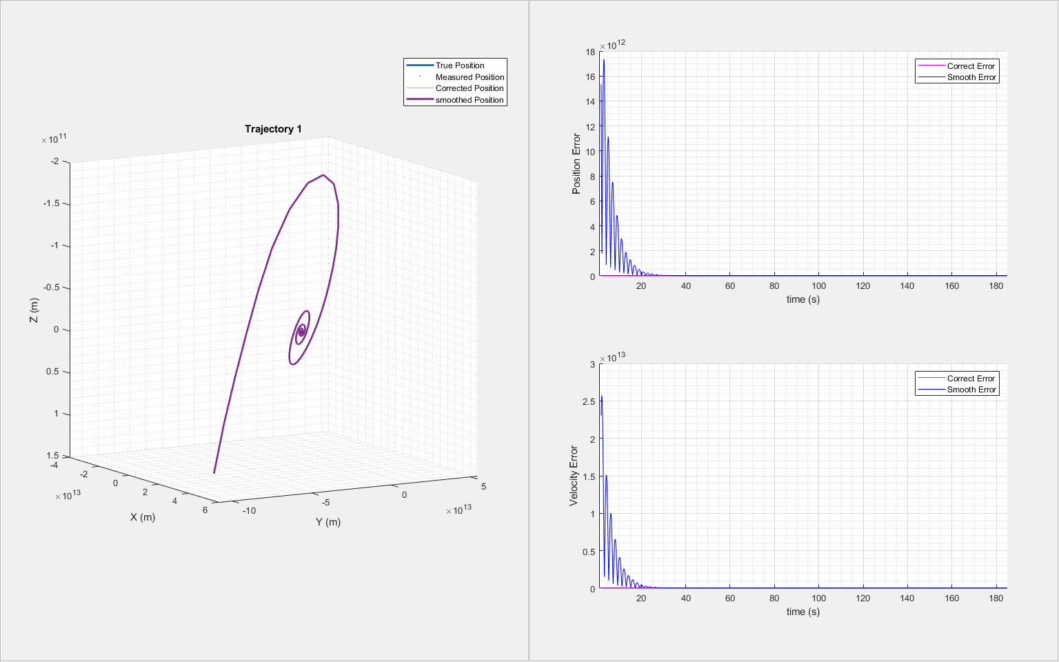
As seen from the results, the smoothing process performs poorly and becomes unstable near 120 seconds. This is mainly due to insufficient process noise in the IMM filter. Rapid changes in aircraft acceleration and sharp turns in short intervals requires higher process noise for the constant acceleration and constant turn motion models of the IMM filter.

Adjusting Process Noise for Better Smoothing Performance

In this section, you adjust the process noise of the filter for better estimation and smoothing results. First, construct a constant velocity, a constant acceleration, and a constant turn-rate model to be used in the IMM filter.

constVelocityEKF = initcvekf(detection);
constantAccelerationEKF = initcaekf(detection);
constantTurnEKF = initctekf(detection);

To compensate the velocity uncertainty, increase the process noise of the constant velocity model in all three axes based on the estimates of the change in the velocity values of the maneuvering target. Similarly, to compensate the acceleration uncertainty, increase the process noise for the constant acceleration model in all three axes based on the estimate of the change in the acceleration values of the maneuvering target. To compensate the turning rate uncertainty, increase the process noise for the turn rate of the constant-turn model.

constantVelocityEKF.ProcessNoise = 36*eye(3,3);
constantAccelerationEKF.ProcessNoise = 100*eye(3,3);
constantTurnEKF.ProcessNoise = 36*eye(4,4);

Create an IMM filter using the three defined estimation filters and enable the smoothing capability.

filters = {constVelocityEKF;constantAccelerationEKF;constantTurnEKF};
imm = trackingIMM(filters,'TransitionProbabilities', 0.99);

imm.EnableSmoothing = true;
imm.MaxNumSmoothingSteps = size(measPosition,1);

Use the filter to estimate the trajectories of six aircraft one-by-one and obtain the smoothed estimates. Visualize the results for each trajectory.

for i = 1:6
    trajNum = i;
    measPosTraj = measPosition(:,:,trajNum);
    [correctState, correctStateCovariance, smoothState, smoothStateCovariance] = helperGenerateSmoothData(clone(imm),measPosTraj,time);
    
    % Visualize the results for each trajectory
    helperTrajectoryViewer(trajNum, time, correctState, smoothState, trueState(:,:,trajNum), measPosTraj)
end

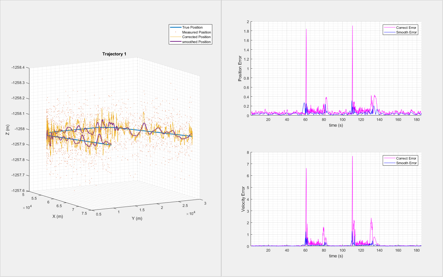
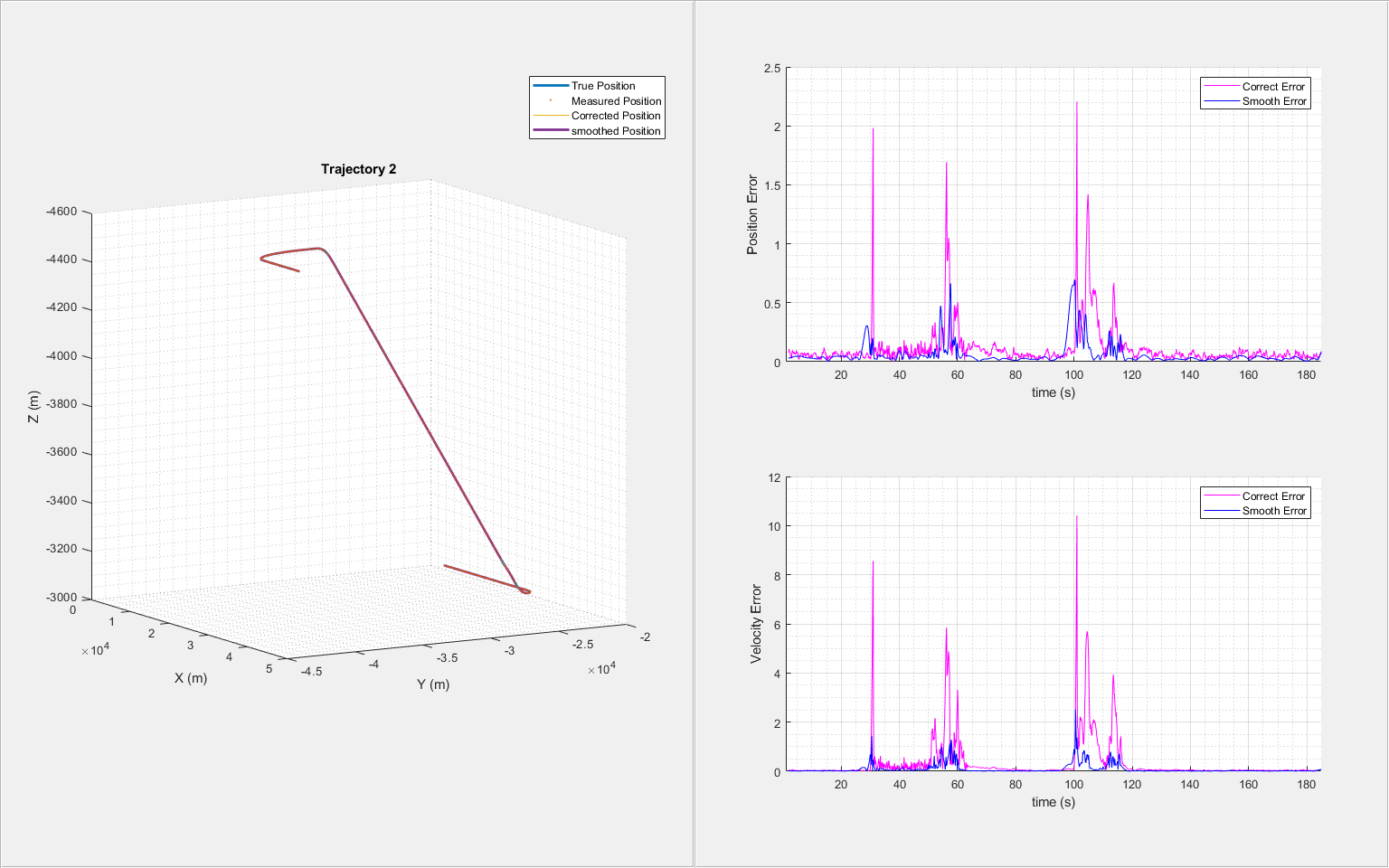
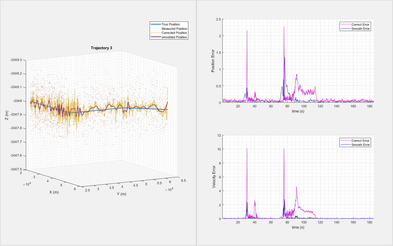
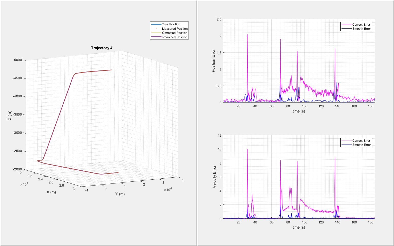
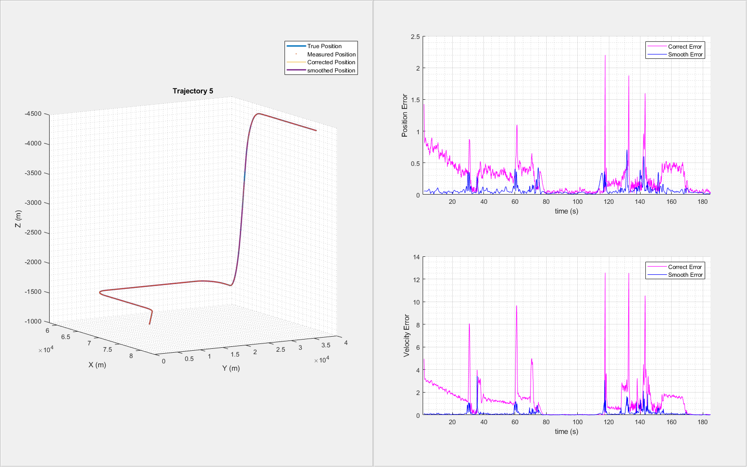
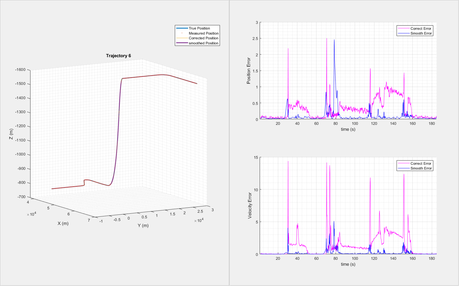
From the results, the use of the adjusted process noise greatly reduces the estimation errors compared with the previous smoothing results without adjusting the process noise.

Summary

In this example, you learned how to smooth filter results to obtain better state estimates. You also learn the importance of adjusting filter noise properly for your specific applications.

Supporting Functions

`helperGenerateCarMeasurements`

Generate measurement inputs for the trajectory of a turning car

function [measPosition, trueState, time] = helperGenerateCarMeasurements()

% Create a trajectory of a car taking a turn.
carWayPoints = [6 2 0; 18 4 0; 25 7 0; 28 10 0; 31 15 0; 33 22 0];
timeSteps = [0 2 4 6 8 10];

% Scenario Generation.

scene = trackingScenario('UpdateRate',20);

plat = platform(scene);
plat.Trajectory = waypointTrajectory(carWayPoints, timeSteps);

% Create trajectory using waypoints from the scenario.
numSteps = 0;
truePosition = [];
trueVelocity = [];
trueAcceleration = [];
time = [];
while advance(scene)
    poses = platformPoses(scene);
    t = scene.SimulationTime;
    numSteps = numSteps + 1;
    truePosition(numSteps,1:3) = poses.Position;
    trueVelocity(numSteps,1:3) = poses.Velocity;
    trueAcceleration(numSteps,1:3) = poses.Acceleration;
    time(numSteps) = t;
end

trueState = [truePosition(:,1,:),trueVelocity(:,1,:),truePosition(:,2,:),trueVelocity(:,2,:),truePosition(:,3,:),trueVelocity(:,3,:)];

% Add measurement noise to true position.
measNoise = 1* randn(size(truePosition));
measPosition = truePosition + [measNoise(:,1:2), zeros(numSteps,1)];

end

helperGenerateAircraftTrajMeasurements

Generate measurement inputs for the trajectories of multiple aircraft

function [measPosition, trueState, time] = helperGenerateAircraftTrajMeasurements()

% Load trajectory waypoints and velocities. The file contains tables of waypoints and 
% velocities (in units of meters and meters per second) that are used to reconstruct six aircraft trajectories.
load('benchmarkTrajectoryTables.mat', 'trajTable');

% Scenario generation.
scene = trackingScenario('UpdateRate',10);

% Assign each platform with a trajectory
for n=1:6
    plat = platform(scene);
    traj = trajTable{n};
    plat.Trajectory = waypointTrajectory(traj.Waypoints, traj.Time, 'Velocities', traj.Velocities);
end

% Create trajectory using waypoints from the scenario.
numSteps = 0;
truePosition = [];
trueVelocity = [];
trueAcceleration = [];
time = [];
while advance(scene)
    poses = platformPoses(scene);
    t = scene.SimulationTime;
    numSteps = numSteps + 1;
    position = vertcat(poses.Position);
    velocity = vertcat(poses.Velocity);
    acceleration = vertcat(poses.Acceleration);
    truePosition(numSteps,1:3,1:6) = permute(position,[3 2 1]);
    trueVelocity(numSteps,1:3,1:6) = permute(velocity,[3 2 1]);
    trueAcceleration(numSteps,1:3,1:6) = permute(acceleration,[3 2 1]);
    time(numSteps) = t;
end
trueState = [truePosition(:,1,:),trueVelocity(:,1,:),truePosition(:,2,:),trueVelocity(:,2,:),truePosition(:,3,:),trueVelocity(:,3,:)];

% Define the measurements to be the position and add normal random noise with a standard deviation of 0.1 to the measurements.
measNoise = 0.1* randn(size(truePosition));
measPosition = truePosition + measNoise;
end

helperGenerateSmoothData

Generate corrected and smoothed states

function [correctState, correctStateCovariance, smoothState, smoothStateCovariance] = helperGenerateSmoothData(imm, measPosTraj, time)

% Output correct and smooth states

numSteps = numel(time);

positionSelector = [1 0 0 0 0 0;0 0 1 0 0 0;0 0 0 0 1 0];
initialState = positionSelector' * measPosTraj(1,:)';
initialCovariance = diag([1,16e4,1,16e4,1,16e4]); % Velocity is not measured
initialize(imm, initialState, initialCovariance);

correctState = zeros(6,numSteps);
correctStateCovariance = zeros(6,6,numSteps);
correctModelProb = zeros(3,numSteps);
correctState(1,1) = measPosTraj(1,1);
correctState(3,1) = measPosTraj(1,2);
correctState(5,1) = measPosTraj(1,3);
correctStateCovariance(:,:,1) = imm.StateCovariance;
correctModelProb(:,1) = imm.ModelProbabilities;

for i = 2:numSteps
    dt = time(i) - time(i-1);
    predict(imm, dt);
    [correctState(:,i), correctStateCovariance(:,:,i)] = correct(imm, measPosTraj(i,:));
    correctModelProb(:,i) = imm.ModelProbabilities;
end

[smoothState, smoothStateCovariance, smoothModelProb] = smooth(imm);

end

`helperTrajectoryViewer`

Visualize smoothing results and compare RMS error

function helperTrajectoryViewer(n, time, correctState, smoothState, trueStateTraj, measPosTraj)

% Create figure and two panels, first panel for position and second panel
% for error visualization

truePosition = trueStateTraj(:,[1 3 5])';
correctPosition = correctState([1 3 5],:);
smoothPosition = smoothState([1 3 5],:);

correctPosError = correctState([1,3,5],1:end-1) - trueStateTraj(1:end-1,[1,3,5])';
smoothPosError = smoothState([1,3,5],:) - trueStateTraj(1:end-1,[1,3,5])';

correctVelError = correctState([2,4,6],1:end-1) - trueStateTraj(1:end-1,[2,4,6])';
smoothVelError = smoothState([2,4,6],:) - trueStateTraj(1:end-1,[2,4,6])';

numSteps = numel(time);

correctPosRMS = zeros(1,numSteps-1);
smoothPosRMS = zeros(1,numSteps - 1);

correctVelRMS = zeros(1,numSteps-1);
smoothVelRMS = zeros(1,numSteps - 1);

for i = 1:numSteps -1
    deltaPc = correctPosError(:,i);
    correctPosRMS(:,i) = sqrt((deltaPc')*deltaPc);
    
    deltaPs = smoothPosError(:,i);
    smoothPosRMS(:,i) = sqrt((deltaPs')*deltaPs);

    
    deltaVc = correctVelError(:,i);
    correctVelRMS(:,i) = sqrt((deltaVc')*deltaVc);
    
    deltaVs = smoothVelError(:,i);
    smoothVelRMS(:,i) = sqrt((deltaVs')*deltaVs);
end

hfig = figure('Name',"Trajectory " + n,'NumberTitle','off','Units','normalized','Position',[0.1 0.1 0.8 0.8]);
hLeftPanel = uipanel(hfig,'Position',[0 0 1/2 1]);
hRightPanel = uipanel(hfig,'Position',[1/2 0 1/2 1]);

xMin = 10*floor(min(truePosition(:,1))/10e3)-5;
xMax = 10*ceil(max(truePosition(:,1))/10e3)+5;
yMin = 10*floor(min(truePosition(:,2))/10e3)-5;
yMax = 10*ceil(max(truePosition(:,2))/10e3)+5;
zMin = 10*floor(min(truePosition(:,3))/10e3)-5;
zMax = 10*ceil(max(truePosition(:,3))/10e3)+5;

% Place x-y plot in left panel for plotting true trajectory, corrected
% trajectory, and smoothed trajectory
hAx1 = axes('Parent',hLeftPanel);
axis(hAx1,[xMin xMax yMin yMax zMin zMax]);
plot3(hAx1,truePosition(1,:),truePosition(2,:),truePosition(3,:),'-','lineWidth',2);
hold on
plot3(hAx1,measPosTraj(:,1),measPosTraj(:,2),measPosTraj(:,3),'.','MarkerSize',3,'lineWidth',2);
plot3(hAx1,correctPosition(1,:),correctPosition(2,:),correctPosition(3,:),'-','lineWidth',.05);
plot3(hAx1,smoothPosition(1,:),smoothPosition(2,:),smoothPosition(3,:),'-','lineWidth',2);

title("Trajectory " + n);
xlabel('X (m)');
ylabel('Y (m)');
zlabel('Z (m)');
lObj = legend('True Position', 'Measured Position', 'Corrected Position', 'smoothed Position','location',"northeast");
axis(hAx1,'square');
grid(hAx1,'minor');
% Switch view to X-Y if Z 0
viewSwitch = mean(truePosition(3,:));
if viewSwitch == 0
    view(90,90);
else
    view(60,10);
end
% Set legend position
legendPos = lObj.Position;
set(lObj,'Position',[legendPos(1)*1.1 legendPos(2) legendPos(3) legendPos(4)])
set(gca,'ZDir','reverse');

% Position RMS plot
hAx2 = subplot(2,1,1,'Parent',hRightPanel);
line(hAx2, time(20:end-1),correctPosRMS(20:end),'color','m');
hold on;
line(hAx2, time(20:end-1),smoothPosRMS(20:end),'color','b');
grid(hAx2,'on');
grid(hAx2,'minor');
xlim([1 inf]);
xlabel('time (s)');
ylabel('Position Error');
legend('Correct Error', 'Smooth Error');

% Velocity RMS plot
hAx3 = subplot(2,1,2,'Parent',hRightPanel);
line(hAx3, time(20:end-1),correctVelRMS(20:end),'color','m');
hold on;
line(hAx3, time(20:end-1),smoothVelRMS(20:end),'color','b');
grid(hAx3,'on');
grid(hAx3,'minor');
xlim([1 inf]);
xlabel('time (s)');
ylabel('Velocity Error');
legend('Correct Error', 'Smooth Error');
end

Smooth Trajectory Estimation of trackingIMM Filter