Track Objects with Wrapping Azimuth Angles and Ambiguous Range and Range Rate Measurements

Track with Angular Measurement Wrapping

When detecting an object, most sensors use a spherical coordinate frame and report the position of the object in azimuth, elevation, and range of the object relative to the sensor. The sensor reports the angular measurements within certain bounds. For example, azimuth angles are often reported within a range of -180 degrees to 180 degrees or 0 degrees to 360 degrees.

While the sensor reports the measurement in spherical coordinates, tracking is usually done in a rectangular frame. To be able to handle the nonlinear transformations required to convert the state from a rectangular frame to a measurement in a spherical frame, a nonlinear filter is required. Some examples of nonlinear filters are the extended Kalman filter and the unscented Kalman filter. For a simple example, consider a filter that maintains a two-dimensional state with positions defined as x and y in the rectangular frame and a sensor that measures position in the two-dimensional plane as azimuth, $\varphi$, and range, r. The conversion from the rectangular state to the measurement, assuming the sensor is located at the origin of the x-y plane is:

For azimuth angles reported in the range of -180 degrees to 180 degrees, if the azimuth angle of the object is close to -180 degrees, the sensor may report an azimuth measurement that wraps around to 180 degrees. These measurements are often referred to as wrapping or circular.

To see that, consider the following results:

% Object is just above the negative x axis
disp(atan2d(1e-5, -100));

  180.0000

% Object is just below the negative x axis
disp(atan2d(-1e-5, -100));

 -180.0000

In the correction step, the Kalman filter uses the residual between the measurement reported by the sensor, $\mathit{z}$, and the measurement expected from the filter state, $\mathit{h}\left(\mathit{x}\right)$, to correct the state estimate:

If an object is located near the wrapping boundary, even if the measurement is relatively accurate, the values of $\mathit{z}$ and $\mathit{h}\left(\mathit{x}\right)$ may be on different sides of the bound, leading to a large residual value. This, in turn, causes the filter to correct the state by a large amount, and may lead the filter to diverge from the accurate state.

The following code uses the azrmeas function, a supporting function attached at the end of this example, to demonstrate filter divergence due to wrapping measurements.

% Initial position
x = -100; 
y = 0;
ekf = trackingEKF(StateTransitionFcn = @constvel, MeasurementFcn = @azrmeas, State = [x;0;y;0]);

% Create a figure
figure(1)
plot(x,y,"r+");
hold on;
grid on;

% Plot the filter estimate on the figure
plot(ekf.State(1), ekf.State(3), "bo");

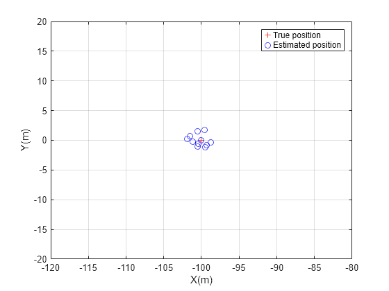
runFilter(ekf, x, y);

From the figure above, the estimated positions diverge significantly from the accurate object position at x = -100 and y = 0.

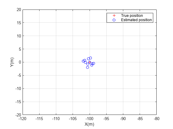
The trackingEKF object provides an ability to handle measurement wrapping by setting the HasMeasurementWrapping property to true. With this specification, the filter uses the second output from the measurement function to get the measurement bounds and wrap the residual within these bounds as proposed in [1]. To support the filter ability to handle measurement wrapping, the function azrmeas has a second output that returns the measurement bounds.

% Initial position
x = -100; 
y = 0;
ekf = trackingEKF(StateTransitionFcn = @constvel, MeasurementFcn = @azrmeas, State = [x;0;y;0], HasMeasurementWrapping = true);

% Create a figure
figure(2)
plot(x,y,"r+");
hold on;
grid on;

% Plot the filter estimate on the figure
plot(ekf.State(1), ekf.State(3), "bo");

runFilter(ekf, x, y);

You use the supporting function, azrmeas, to obtain the foregoing results. You can also use the built-in measurement and filter initialization functions to handle measurement wrapping and get the same results. The following code block shows the equivalent workflow to use built-in functions.

% Initialize the filter with a detection in spherical coordinates
mp = struct(Frame = "Spherical", HasElevation = false, HasVelocity = false);
detection = objectDetection(0, [-180;100], MeasurementParameters = mp);
ekf = initcvekf(detection);

% Create a figure
figure(3)
plot(x,y,"r+");
hold on;
grid on;

% Plot the filter estimate on the figure
plot(ekf.State(1), ekf.State(3), "bo");

runFilter(ekf, x, y, mp);

Radar Range and Range Rate Ambiguities

So far, the measurement wrapping was due to the way format that the sensor reports angle but had nothing to do with how the sensor processes its measurement. This section focuses on a different source of measurement wrapping in radars: the process the radar measures range and range rate of an object.

To measure range, the radar emits a pulse of radio frequency waves, which propagates at the speed of light, c. After the pulse is reflected from the object, it travels back to the radar. The radar measures the time difference between the arrival time and the pulse emission time, $$\tau$$. For a monostatic radar, in which the radar pulse travels to the object and back to the radar, the distance that the pulse traveled is twice the range to the object.

The radar repeats the pulses at a certain frequency, called the pulse repetition frequency (PRF). To be able to unambiguously determine which pulse corresponds to the return from the object, the return must arrive at the radar before the emission of the next pulse. The maximum distance that the radar can unambiguously determine using the returned pulse is called the maximum unambiguous range, defined as:

From the expression, to be able to unambiguously measure larger ranges, the radar needs to have a low PRF.

In addition, to measure the object velocity along the range axis from the radar, known as range rate, the radar uses the Doppler effect. The Doppler effect shifts the frequency observed by the radar when the target moves in a direction along the vector to the radar. This shift must be within the radar pulse repetition frequency. Therefore, the range rate measurement is unambiguous in the interval:

where, f is the frequency of the radio waves. From the expression, to be able to unambiguously measure high range rates, the PRF must be high.

Obviously, there is a contradiction between the PRF needed for long range measurements, which must be low, and the PRF needed for high velocity measurements, which must be high. In many cases, a compromise is made by choosing a medium PRF, which is selected based on the required maximum range and the maximum expected object speed. However, if the object is either located farther from the radar or moves faster than expected, the radar reports an ambiguous range or an ambiguous range rate according to the following:

For example, if a radar has a maximum unambiguous range of 100 km, but the target is located at a range of 110 km from the radar, the radar reports a range of 10 km.

A few techniques can be used to improve the maximum unambiguous range and the maximum unambiguous range rate using signal processing techniques. For example, radar engineers sometimes use the crt (Phased Array System Toolbox) if the radar uses multiple PRFs.

To summarize, while angle wrapping is caused by the bounding of angle measurements to a certain range, range and range rate wrapping are caused by the radar inherent mode of operation. Even when signal processing techniques are used to improve the range and range rate ambiguities, some ambiguities still happen and must be handled by the estimation filter and the multi-object tracking algorithms.

Estimate Object Position with Range or Range Rate Ambiguities

In this section, you use an extended Kalman filter to estimate the position of an object that is moving away from the radar and crosses over the maximum unambiguous range. You must first define a measurement function that reports the range bounds, in this case the function azrmeas100, attached as a supporting function at the end of this example. This function is similar to the function azrmeas used in the previous sections except that the maximum range is bounded to 100.

% Initial position
r = 70; % Range from radar, in m
rr = 10; % Range rate, the object moves away from the radar at 10 m/s
az = 10; % The azimuth angle to the object is 10 degrees
[x,y] = pol2cart(deg2rad(az),r);
ekf = trackingEKF(StateTransitionFcn = @constvel, MeasurementFcn = @azrmeas100, State = [x;0;y;0], HasMeasurementWrapping = true);

% Create a figure
figure(4)
th = plot(x,y,"r+");
hold on;
axis equal
axis([0 220 -120 120])
xlabel("X(m)");
ylabel("Y(m)");

% Plot the reported position
rh = plot(x,y,"kx");

% Plot the estimated position
eh = plot(ekf.State(1), ekf.State(3), "bo");
grid on;

% Add the maximum unambiguous range circle
rectangle(Position = [-100 -100 200 200], Curvature = [1 1], LineStyle = "--", EdgeColor = "r");
text(75, 80, "Maximum" + newline + "Unambiguous" + newline + "Range");

hold off
legend("True position", "Reported position", "Estimated position", Location = "southeast");

% Use the same seed
rng(0,"twister");

dt = 0.2;
for time = dt:dt:8
    predict(ekf,1);

    % Move the object
    r = r + rr * dt;
    [x,y] = pol2cart(deg2rad(az),r);
    set(th, XData = x, YData = y)

    % Measurement with some noise
    z = [az;r] + 0.1 * randn(2,1);

    % Wrap the azimuth measurement in the range -180 to 180 and the radius
    % in the range 0 to 100
    z(1) = mod(z(1)+180, 360) - 180;
    z(2) = mod(z(2),100);

    % Plot the reported position
    [x,y] = pol2cart(deg2rad(z(1)),z(2));
    set(rh, XData = x, YData = y);

    % Correct the filter with the measurement
    correct(ekf,z);

    % Plot the filter estimate on the figure
    set(eh, XData = ekf.State(1), YData = ekf.State(3));

    drawnow
end

You can observe that the filter was able to estimate the position of the object even when the object exceeds the maximum unambiguous range.

Multi-Object Tracking in the Presence of Angular and Range Ambiguities

When tracking multiple objects, the tracker has to assign the measurement to the correct object even if the reported measurement was wrapped, in addition to estimating the dynamics of each object. This section shows how to use multiobject trackers to track three objects, where each object causes the radar to report measurements that wrap in range, range rate, or azimuth.

The following code creates a radar that covers 360 degrees around the radar without scanning. The radar has a maximum unambiguous range of 100 meters and has a maximum unambiguous range rate of 12 meters per second. You mount the radar on a platform.

scenario = trackingScenario(UpdateRate = 0);
radar = fusionRadarSensor( ...
    SensorIndex = 1, ...
    ScanMode = "No scanning", ...
    UpdateRate = 10, ...
    FieldOfView = [360;10], ...
    HasElevation = false, ...
    HasRangeRate = true, ...
    HasRangeAmbiguities = true, ...
    HasRangeRateAmbiguities = true, ...
    AzimuthResolution = 0.1, ...
    ReferenceRange = 100, ...
    RangeResolution = 1, ...
    RangeRateResolution = 1, ...
    HasFalseAlarms = false, ...
    HasINS = true, ...
    DetectionCoordinates = "Sensor Spherical",...
    MaxUnambiguousRange = 100,...
    MaxUnambiguousRadialSpeed = 12);
platform(scenario, sensors = radar);

You define the trajectories of the three objects. The first object begins its motion about half the distance to the radar maximum unambiguous range, continues moving away, and eventually crosses the maximum unambiguous range. The second object begins its motion with a relatively low speed but then accelerates to a range rate that is above the maximum unambiguous range rate of the radar. The third object begins its motion just above the negative x axis and moves down, crossing the x axis where the azimuth measurement wraps. In practice, some objects may give rise to measurements with all three ambiguities.

traj1 = waypointTrajectory([50 10 0; 130 20 0], [0;10]); % Across the range ambiguity
platform(scenario, Trajectory = traj1);
traj2 = waypointTrajectory([60 -20 0; 40 0 0; -60 60 0], [0;3;10]); % Faster than the range rate ambiguity
platform(scenario, Trajectory = traj2);
traj3 = waypointTrajectory([-70 10 0; -70 -10 0], [0;10]); % Across the azimuth wrapping
platform(scenario, Trajectory = traj3);

You visualize the scenario using the createVisualization supporting function.

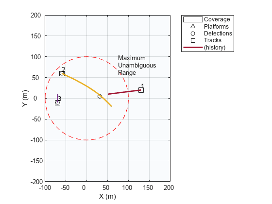
[plp, detp, trkp] = createVisualization(scenario);

You use the trackerGNN object with a constant velocity extended Kalman filter to track the objects. The built-in initcvekf initialization function uses the constant velocity measurement function, cvmeas, which supports azimuth wrapping, but does not support range or range rate wrapping, because they are radar specific. Therefore, you modify the filter initialization function and add a measurement function that supports range and range rate wrapping. You can see the details of the initBoundedCVEKF and boundedCVMeas functions in the Supporting Functions section.

tracker = trackerGNN(FilterInitializationFcn = @initBoundedCVEKF);
positionSelector = [1 0 0 0 0 0; 0 0 1 0 0 0; 0 0 0 0 1 0];

Run the simulation and track the objects.

while advance(scenario)
    % Simulation time
    time = scenario.SimulationTime;

    % Collect all the detections from the scenario and plot them
    detections = detect(scenario);
    detPositions = getDetectionPositions(detections);
    plotDetection(detp, detPositions);

    % Update the tracker and plot the tracks
    tracks = tracker(detections, time);
    [pos,cov] = getTrackPositions(tracks,positionSelector);
    trIDs = string([tracks.TrackID]);
    plotTrack(trkp, pos, cov, trIDs);
end

You observe that the tracker is able to track all three objects even though the measurements reported by the radar are wrapping in azimuth, range, and range rate.

Summary

This example shows how to track with wrapped measurements. Sensors often report angular measurements that wrap due to the angle circular nature, which is common to all sensors. In addition, due to the way radars operate, their measurements can have ambiguity in range and in range rate, which is specific to each radar. You saw how to define nonlinear filters that can handle wrapping measurements. The nonlinear filters require a measurement function that provides the measurement bounds. For angular measurement wrapping, the built-in measurement functions, such as cameas, cvmeas, ctmeas, singermeas, and cvmeasmsc provide the default azimuth and elevation bounds. To handle measurement wrapping in range and range rate, you must define the radar specific bounds, as shown in this example. Finally, this example showed how the multi-object trackers, when configured with tracking filters and measurement functions that report the measurement bounds, can track objects even in the presence of wrapping measurements.

References

[1] Crouse David Frederic, "Cubature/unscented/sigma point Kalman filtering with angular measurement models," 2015 18th International Conference on Information Fusion (Fusion), Washington DC, 2015, pp. 1550–1557.

Supporting Functions

azrmeas

This function provides the azimuth and range measurement without bounds.

function [z, bounds] = azrmeas(state)
x = state(1);
y = state(3);
az = atan2d(y,x);
r = sqrt(x^2 + y^2);
z = [az;r];
bounds = [-180 180; -inf inf];
end

runFilter

The function runs the filter for wrapped angular measurement cases.

function runFilter(filter, x, y, mp)
% Use a constant random number generator seed
rng(0,"v4");

for step = 1:10
    predict(filter,1);

    % Measurement with some noise
    z = azrmeas([x;0;y;0]) + randn(2,1);

    % Wrap the azimuth measurement in the range -180 to 180
    z(1) = mod(z(1)+180, 360) - 180;

    % Correct the filter with the measurement
    if nargin < 4
        correct(filter,z);
    else
        correct(filter, z, mp);
    end

    % Plot the filter estimate on the figure
    plot(filter.State(1), filter.State(3), "bo");
end
hold off
legend("True position", "Estimated position")
xlabel("X(m)");
ylabel("Y(m)");

if filter.HasMeasurementWrapping
    axis([-120 -80 -20 20]);
else
    axis([-200 500 -200 500]);
end
snapnow
end

azrmeas100

This function provides the azimuth and range measurements. Range is bounded between 0 and 100.

function [z, bounds] = azrmeas100(state)
x = state(1);
y = state(3);
az = atan2d(y,x);
r = mod(sqrt(x^2 + y^2), 100);
z = [az;r];
bounds = [-180 180; 0 100];
end

boundedCVMeas

The function is similar to cvmeas with range measurement bounded between 0 and 100 and range rate bounded between -12 and 12.

function [z, bounds] = boundedCVMeas(state, varargin)
% Use the regular cvmeas to get the measurement and bounds
mp = varargin{1};
[z, bounds] = cvmeas(state, mp);

% Add the range ambiguity and range rate ambiguity to the bounds
if mp(1).HasRange
    rangeIndex = mp(1).HasAzimuth + mp(1).HasElevation + mp(1).HasRange;
    bounds(rangeIndex, :) = [0 100];
    if mp(1).HasVelocity % Range rate can only be reported if range is reported
        bounds(rangeIndex + 1, :) = [-12 12];
    end
end
end

initBoundedCVEKF

Filter initialization function for a constant velocity extended Kalman filter that uses the boundedCVMeas measurement function.

function ekf = initBoundedCVEKF(detection)
% Use the regular initcvekf to get the filter
ekf = initcvekf(detection);
ekf.MeasurementFcn = @boundedCVMeas;
end

createVisualization

A helper function to create the visualization used in this example. The function returns the handles to the platform plotter, detection plotter, and track plotter.

function [plp, detp, trkp] = createVisualization(scenario)
tp = theaterPlot(Xlimits = [-100 200], YLimits = [-200 200], ZLimits = [-50 50]);
cvp = coveragePlotter(tp, DisplayName = "Coverage", Tag = "Radar", Alpha = [0.01 0.1]);
plotCoverage(cvp, coverageConfig(scenario));
plp = platformPlotter(tp, DisplayName = "Platforms", Tag = "Platforms");
trajp = trajectoryPlotter(tp);
positions = cell(numel(scenario.Platforms)-1,1);
for i = 2:numel(scenario.Platforms)
    traj = scenario.Platforms{i}.Trajectory;
    ts = (traj.TimeOfArrival(1):(traj.TimeOfArrival(end)-traj.TimeOfArrival(1))/100:traj.TimeOfArrival(end));
    positions{i-1} = lookupPose(traj,ts);
end
plotTrajectory(trajp,positions);
detp = detectionPlotter(tp, DisplayName = "Detections", Tag = "Detections");
trkp = trackPlotter(tp, DisplayName = "Tracks", Tag = "Tracks", ConnectHistory = "on", ColorizeHistory = "on");

% Add the maximum unambiguous range circle
rectangle(Position = [-100 -100 200 200], Curvature = [1 1], LineStyle = "--", EdgeColor = "r");
text(75, 80, "Maximum" + newline + "Unambiguous" + newline + "Range");
grid on
end

getDetectionPositions

A helper function to return the detection positions for measurements in spherical coordinates relative to a sensor at the origin.

function detPositions = getDetectionPositions(detections)
numDets = numel(detections);
detPositions = zeros(numDets,3);
for i = 1:numDets
    mp = detections{i}.MeasurementParameters(1);
    if mp.HasAzimuth
        az = deg2rad(detections{i}.Measurement(1));
    else
        az = 0;
    end
    if mp.HasElevation
        el = deg2rad(detections{i}.Measurement(1 + mp.HasAzimuth));
    else
        el = 0;
    end
    if mp.HasRange
        r = detections{i}.Measurement(1 + mp.HasAzimuth + mp.HasElevation);
    else
        r = 0;
    end
    [x, y, z] = sph2cart(az, el, r);
    detPositions(i,:) = [x, y, z];
end
end