粒子群输出函数

此示例显示如何使用 particleswarm 的输出函数。输出函数绘制了粒子在每个维度上占据的范围。

求解器每次迭代后都会运行一个输出函数。有关语法详细信息以及输出函数可用的数据，请参阅输出函数和绘图函数。

自定义绘图函数

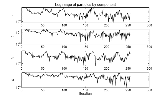
本示例末尾的 pswplotranges 辅助函数绘制了一个每维一条线的图。每条线代表该维度中群粒子的范围。该图采用对数尺度来适应较宽的范围。如果群收敛到一个点，那么每个维度的范围都会变为零。但如果群没有收敛到单个点，那么范围在某些维度上就会远离零。

目标函数

本例末尾的 multirosenbrock 辅助函数将罗森布洛克函数推广到任意偶数维。它在点 0 处具有全局最小值 [1,1,1,1,...]。

设置并运行问题

将 multirosenbrock 函数设置为目标函数。使用四个变量。为每个变量设置一个下界 -10 和一个上界 10。

fun = @multirosenbrock;
nvar = 4; % A 4-D problem
lb = -10*ones(nvar,1); % Bounds to help the solver converge
ub = -lb;

设置选项以使用输出函数。

options = optimoptions(@particleswarm,'OutputFcn',@pswplotranges);

为了获得可再现的结果，请设置随机数生成器。然后调用求解器。

rng default % For reproducibility
[x,fval,eflag] = particleswarm(fun,nvar,lb,ub,options)

Figure pranges contains 4 axes objects. Axes object 1 with title Log range of particles by component, ylabel 1 contains an object of type line. Axes object 2 with ylabel 2 contains an object of type line. Axes object 3 with ylabel 3 contains an object of type line. Axes object 4 with xlabel Iteration, ylabel 4 contains an object of type line.

Optimization ended: relative change in the objective value 
over the last OPTIONS.MaxStallIterations iterations is less than OPTIONS.FunctionTolerance.

x = 1×4

    0.9964    0.9930    0.9835    0.9681

fval = 
3.4935e-04

eflag = 
1

结果

求解器返回最优 [1,1,1,1] 附近的一个点。但是群的跨度不会收敛到零。

辅助函数

以下代码创建 pswplotranges 辅助函数。

function stop = pswplotranges(optimValues,state)

stop = false; % This function does not stop the solver
switch state
    case 'init'
        fig = figure();
        set(fig,'numbertitle','off','name','pranges')
        nplot = size(optimValues.swarm,2); % Number of dimensions
        for i = 1:nplot % Set up axes for plot
            subplot(nplot,1,i);
            tag = sprintf('psoplotrange_var_%g',i); % Set a tag for the subplot
            semilogy(optimValues.iteration,0,'-k','Tag',tag); % Log-scaled plot
            ylabel(num2str(i))
        end
        xlabel('Iteration','interp','none'); % Iteration number at the bottom
        subplot(nplot,1,1) % Title at the top
        title('Log range of particles by component')
        setappdata(gcf,'t0',tic); % Set up a timer to plot only when needed
    case 'iter'
        fig = findobj(0,'Type','figure','Name','pranges');
        set(0,'CurrentFigure',fig);
        nplot = size(optimValues.swarm,2); % Number of dimensions
        for i = 1:nplot
            subplot(nplot,1,i);
            % Calculate the range of the particles at dimension i
            irange = max(optimValues.swarm(:,i)) - min(optimValues.swarm(:,i));
            tag = sprintf('psoplotrange_var_%g',i);
            plotHandle = findobj(get(gca,'Children'),'Tag',tag); % Get the subplot
            xdata = plotHandle.XData; % Get the X data from the plot
            newX = [xdata optimValues.iteration]; % Add the new iteration
            plotHandle.XData = newX; % Put the X data into the plot
            ydata = plotHandle.YData; % Get the Y data from the plot
            newY = [ydata irange]; % Add the new value
            plotHandle.YData = newY; % Put the Y data into the plot
        end
        if toc(getappdata(gcf,'t0')) > 1/30 % If 1/30 s has passed
          drawnow % Show the plot
          setappdata(gcf,'t0',tic); % Reset the timer
        end
    case 'done'
        % No cleanup necessary
end
end

以下代码创建 multirosenbrock 辅助函数。

function F = multirosenbrock(x)
% This function is a multidimensional generalization of Rosenbrock's
% function. It operates in a vectorized manner, assuming that x is a matrix
% whose rows are the individuals.

% Copyright 2014 by The MathWorks, Inc.

N = size(x,2); % assumes x is a row vector or 2-D matrix
if mod(N,2) % if N is odd
    error('Input rows must have an even number of elements')
end

odds  = 1:2:N-1;
evens = 2:2:N;
F = zeros(size(x));
F(:,odds)  = 1-x(:,odds);
F(:,evens) = 10*(x(:,evens)-x(:,odds).^2);
F = sum(F.^2,2);
end

另请参阅

主题

输出函数和绘图函数