六元件八木天线的替代优化

此示例使用:

此示例说明如何使用替代优化求解器优化天线设计。天线的辐射模式敏感地取决于定义天线形状的参数。通常，辐射模式的特征具有多个局部最优解。为了计算辐射模式，本例使用了 Antenna Toolbox™ 函数。

八木宇田天线是一种广泛用于商业和军事领域各种应用的辐射结构体。该天线可以接收 VHF-UHF 频率范围内的电视信号[1]。八木宇田天线是一种定向行波天线，具有单个驱动元件，通常是一个折叠偶极子或标准偶极子，周围环绕着几个无源偶极子。无源元件构成反射器和引向器。这些名称标识了相对于驱动元素的位置。反射器偶极子位于驱动元件后面，位于天线辐射后瓣的方向上。引向器偶极子位于驱动元件的前方，沿着主光束形成的方向。

设计参数

指定 VHF 频段中心的初始设计参数[2]。

freq = 165e6;
wirediameter = 19e-3;
c = physconst("lightspeed");
lambda = c/freq;

创建八木天线

八木宇田天线的驱动元件是折叠偶极子，这是此类天线的标准激励器。调整折叠偶极子的长度和宽度参数。因为圆柱形结构体被建模为等效金属条，所以使用 Antenna Toolbox™ 中提供的 cylinder2strip 实用函数来计算宽度。设计频率下的长度为 $λ / 2$ 。

d = dipoleFolded;
d.Length = lambda/2;
d.Width = cylinder2strip(wirediameter/2);
d.Spacing = d.Length/60;

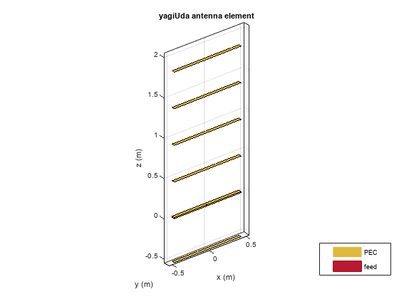
创建八木宇田天线，以激励器为折叠偶极子。将反射器和引向器元素的长度设置为 $λ / 2$ 。将引向器数量设置为四。将反射器和引向器间距分别指定为 $0.3 λ$ 和 $0.25 λ$ 。这些设置提供了初步猜测并作为优化过程的起点。展示初始设计。

Numdirs = 4;
refLength = 0.5;
dirLength = 0.5*ones(1,Numdirs);
refSpacing = 0.3;
dirSpacing = 0.25*ones(1,Numdirs);
initialdesign = [refLength dirLength refSpacing dirSpacing].*lambda;
yagidesign = yagiUda;
yagidesign.Exciter = d;
yagidesign.NumDirectors = Numdirs;
yagidesign.ReflectorLength = refLength*lambda;
yagidesign.DirectorLength = dirLength.*lambda;
yagidesign.ReflectorSpacing = refSpacing*lambda;
yagidesign.DirectorSpacing = dirSpacing*lambda;
show(yagidesign)

Figure contains an axes object. The axes object with title yagiUda antenna element, xlabel x (m), ylabel y (m) contains 5 objects of type patch, surface. These objects represent PEC, feed.

绘制设计频率下的辐射图

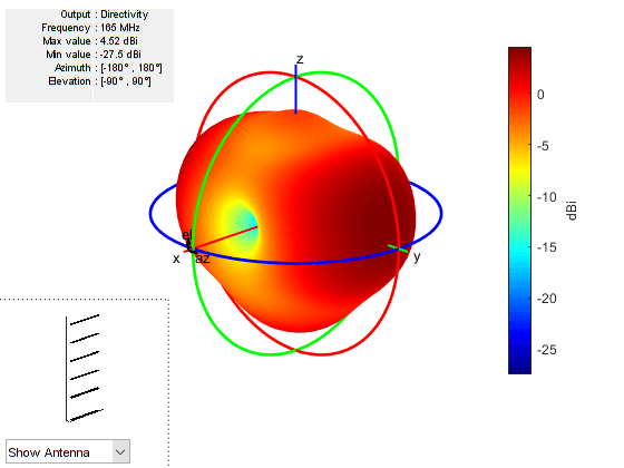
在执行优化过程之前，以 3-D 形式绘制初始猜测的辐射模式。

fig1 = figure;
pattern(yagidesign,freq);

Figure contains an axes object and other objects of type uicontrol. The axes object contains 5 objects of type patch, surface.

该天线在首选方向（天顶（仰角 = 90 度））没有更高的方向性。最初的八木天线设计是一个设计很差的辐射器。

设置优化

使用以下变量作为优化的控制变量：

反射器长度（1 个变量）
引向器长度（4 个变量）
反射器间距（1 个变量）
引向器间距（4 个变量）

就单个向量参数 parasiticVals 而言，使用以下设置：

反射器长度 = parasiticVals(1)
引向器长度 = parasiticVals(2:5)
反射器间距 = parasiticVals(6)
引向器间距 = parasiticVals(7:10)

就 parasiticVals 而言，设置一个目标函数，旨在在 90 度方向上具有较大值，在 270 度方向上具有较小值，并且在仰角波束宽度角度边界之间具有较大最大功率值。

type yagi_objective_function2.m

function objectivevalue = yagi_objective_function2(y,parasiticVals,freq,elang)
% yagi_objective_function2 returns the objective for a 6-element Yagi
% objective_value = yagi_objective_function(y,parasiticvals,freq,elang)
% assigns the appropriate parasitic dimensions, parasiticvals, to the Yagi
% antenna y, and uses the frequency freq and angle pair elang to calculate
% the objective function value.

% The yagi_objective_function2 function is used for an internal example.
% Its behavior might change in subsequent releases, so it should not be
% relied upon for programming purposes.

% Copyright 2014-2018 The MathWorks, Inc.

bw1 = elang(1);
bw2 = elang(2);
y.ReflectorLength = parasiticVals(1);
y.DirectorLength = parasiticVals(2:y.NumDirectors+1);
y.ReflectorSpacing = parasiticVals(y.NumDirectors+2);
y.DirectorSpacing = parasiticVals(y.NumDirectors+3:end);
output = calculate_objectives(y,freq,bw1,bw2);
output = output.MaxDirectivity + output.FB;
objectivevalue= -output; % To maximize
end

function output = calculate_objectives(y,freq,bw1,bw2)
%calculate_objectives calculate the objective function
% output = calculate_objectives(y,freq,bw1,bw2) Calculate the directivity
% in az = 90 plane that covers the main beam, sidelobe and backlobe.
% Calculate the maximum directivity, sidelobe level and backlobe and store
% in fields of the output variable structure.
[es,~,el] = pattern(y,freq,90,0:1:270);   
el1 = el < bw1;                           
el2 = el > bw2;                           
el3 = el>bw1&el<bw2;
emainlobe = es(el3);
esidelobes =([es(el1);es(el2)]);
Dmax = max(emainlobe);
SLLmax = max(esidelobes);
Backlobe = es(end);
F = es(91);
B = es(end);
F_by_B = F-B;
output.MaxDirectivity= Dmax;
output.MaxSLL = SLLmax;
output.BackLobeLevel = Backlobe;
output.FB = F_by_B;
end

设置控制变量的边界。

refLengthBounds = [0.4;
                    0.6];
dirLengthBounds = [0.35 0.35 0.35 0.35;   % lower bound on director length
                   0.495 0.495 0.495 0.495];  % upper bound on director length
refSpacingBounds = [0.05;                 % lower bound on reflector spacing
                    0.30];                % upper bound on reflector spacing
dirSpacingBounds = [0.05 0.05 0.05 0.05;  % lower bound on director spacing
                    0.23 0.23 0.23 0.23]; % upper bound on director spacing
                
LB = [refLengthBounds(1) dirLengthBounds(1,:) refSpacingBounds(1) dirSpacingBounds(1,:) ].*lambda;
UB = [refLengthBounds(2) dirLengthBounds(2,:) refSpacingBounds(2) dirSpacingBounds(2,:) ].*lambda;

设置优化的初始点，并设置仰角波束宽度角度边界。

parasitic_values = [ yagidesign.ReflectorLength,                        ...
                     yagidesign.DirectorLength,                         ...
                     yagidesign.ReflectorSpacing                        ...
                     yagidesign.DirectorSpacing];                

elang = [60 120];                   % elevation beamwidth angles at az = 90

替代优化

为了寻找目标函数的全局最优，使用 surrogateopt 作为求解器。设置选项以允许 500 次函数计算、包括初始点、使用并行计算以及使用 'surrogateoptplot' 绘图函数。要了解 'surrogateoptplot' 图，请参阅解释 surrogateoptplot...

surrogateoptions = optimoptions("surrogateopt", MaxFunctionEvaluations=500,...
    InitialPoints=parasitic_values, UseParallel=canUseGPU(), PlotFcn="surrogateoptplot");
rng(4) % For reproducibility
optimdesign = surrogateopt(@(x) yagi_objective_function2(yagidesign,x,freq,elang),...
                      LB,UB,surrogateoptions);

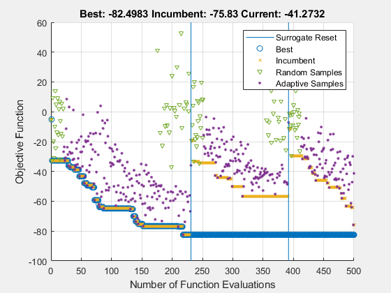
Figure Optimization Plot Function contains an axes object. The axes object with title Best: -82.4983 Incumbent: -75.83 Current: -41.2732, xlabel Number of Function Evaluations, ylabel Objective Function contains 6 objects of type line. One or more of the lines displays its values using only markers These objects represent Best, Incumbent, Random Samples, Adaptive Samples, Surrogate Reset.

surrogateopt stopped because it exceeded the function evaluation limit set by 
'options.MaxFunctionEvaluations'.

surrogateopt 找到一个目标函数值为 -82.5 的点。研究优化参数对天线辐射模式的影响。

绘制优化模式

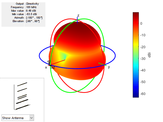
绘制设计频率下的优化天线模式。

yagidesign.ReflectorLength = optimdesign(1);
yagidesign.DirectorLength = optimdesign(2:5);
yagidesign.ReflectorSpacing = optimdesign(6);
yagidesign.DirectorSpacing  = optimdesign(7:10);
fig2 = figure;
pattern(yagidesign,freq)

Figure contains an axes object and other objects of type uicontrol. The axes object contains 5 objects of type patch, surface.

显然，天线现在在天顶辐射的功率明显更大。

E 平面和 H 平面图案切割

为了更好地了解两个正交平面中的行为，绘制 E 平面和 H 平面中电场的归一化幅度，即方位角分别 = 0 和 90 度。

fig3 = figure;
pattern(yagidesign,freq,0,0:1:359);

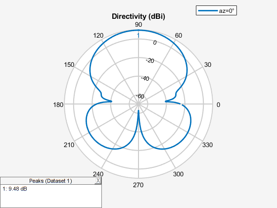
Figure contains an object of type uicontainer.

fig4 = figure;
pattern(yagidesign,freq,90,0:1:359);

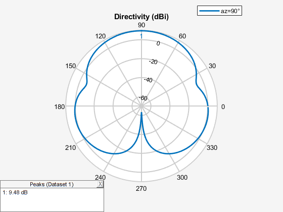
Figure contains an object of type uicontainer.

优化的设计使辐射模式有显著的改善。在朝向天顶的所需方向上可实现更高的方向性。后瓣较小，导致该天线具有良好的前后比。计算天顶的方向性、前后比以及 E 平面和 H 平面的波束宽度。

D_max = pattern(yagidesign,freq,0,90)

D_max = 9.4799

D_back = pattern(yagidesign,freq,0,-90)

D_back = -63.5385

F_B_ratio = D_max - D_back

F_B_ratio = 73.0184

Eplane_beamwidth = beamwidth(yagidesign,freq,0,1:1:360)

Eplane_beamwidth = 56.0000

Hplane_beamwidth = beamwidth(yagidesign,freq,90,1:1:360)

Hplane_beamwidth = 72

与制造商数据表的比较

优化后的八木天线实现了 9.48 dBi 的前向方向性，相当于 7.4 dBd（相对于偶极子）。这个结果比参考文献[2]数据表报告的增益值(8.5 dBd)略小。前后比为 73 dB；这是优化器最大化的量的一部分。优化后的八木宇田天线的 E 平面波束宽度为 56 度，与数据表相同。优化后的八木宇田天线的 H 平面波束宽度为 72 度，而数据表上的值为 63 度。该示例并未解决频带内的阻抗匹配问题。

制表初始设计和优化设计

将初始设计猜测和最终优化设计值制成表格。

yagiparam=  {'Reflector Length';
             'Director Length - 1'; 'Director Length - 2';
             'Director Length - 3'; 'Director Length - 4';
             'Reflector Spacing';   'Director Spacing - 1';
             'Director Spacing - 2';'Director Spacing - 3';
             'Director Spacing - 4'};         
initialdesign = initialdesign';
optimdesign = optimdesign';
T = table(initialdesign,optimdesign,RowNames=yagiparam)

T=10×2 table
                            initialdesign    optimdesign
                            _____________    ___________

    Reflector Length           0.90846          1.0009  
    Director Length - 1        0.90846         0.66951  
    Director Length - 2        0.90846         0.71935  
    Director Length - 3        0.90846         0.73777  
    Director Length - 4        0.90846         0.75073  
    Reflector Spacing          0.54508         0.32285  
    Director Spacing - 1       0.45423         0.23736  
    Director Spacing - 2       0.45423        0.090846  
    Director Spacing - 3       0.45423         0.37511  
    Director Spacing - 4       0.45423         0.33403