Compressor Map
This example shows how to create the pressure ratio, corrected mass flow rate, and efficiency tables required to specify the performance characteristics of a dynamic compressor.
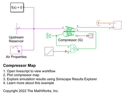
open_system('CompressorMap')
Using a Compressor Map
Compressor maps are M-by-N matrices where the number of rows, M, is equal to the number of corrected speeds and the number of columns, N, is equal to the number of points along each corrected speed line. The indexing vectors for these matrices are a corrected speed vector of length M and a vector for the auxiliary coordinate system parameter β of length N with values ranging from 0 to 1.
This figure shows a compressor map. In this example, you use this compressor map to parameterize a Compressor (G) block.

Extracting Compressor Map Data
To use the data in a compressor block to parameterize a Simscape™ compressor block, convert the map data into numerical values and organize the information contained in the map image. Use the Graph Data Extractor app to import the data from the compressor map. Pull the data in two separate tasks:
Extract the corrected mass flow rate and pressure ratio data of the compressor by selecting points along each constant-speed line.
Collect the compressor efficiency data by selecting points for each efficiency level. This data is a collection of corrected mass flow rate and pressure ratio points valid for a given efficiency. You will then interpolate this data to be consistent with the data gathered in task 1.
To ensure that the data sets are rectangular matrices that do not have any empty entries, select the same number of points for each constant speed line and each efficiency level. However, the number of points for the speed lines and efficiency levels do not have to be the same.
Extract Flow and Pressure Ratio Values from Constant-Speed Lines
Using the Graph Data Extractor app, load the compressor map image and identify the axes scaling. For each constant-speed line, select the same number of points. Sample the points counter-clockwise along each speed line, starting at the choke line, if applicable, and ending on the surge line, which is the dotted red line. This image shows the selected points for the data at 2500 rpm.
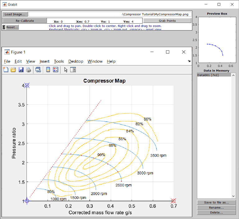
Space the selected points as uniformly as possible. The more regular the grid of flow and pressure ratio points within the defined map space, the more smoothly you can interpolate the map, both for defining efficiency and for use with the Simscape compressor. Select data points for all of the constant-speed lines you want to be part of the compressor map. Export the data from the Graph Data Extractor app and save it as a MAT file.
Collect Efficiency Contours
Using the Graph Data Extractor app, create MAT files containing the corrected mass flow rate and pressure ratio data for each efficiency contour level. You do not need to select the points in a specific order or start at a specific point, but it is recommended to select points in a clockwise or counter-clockwise direction. This image shows the selected points for the 80% efficiency contour.
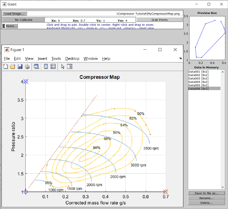
Select all contour points. There can be breaks in the contour lines. Do not add fictitious points. The Graph Data Extractor app automatically sorts and connects the points based on the x-value regardless of the order you selected them in, but this does not impact the imported map data.
Export the data from the Graph Data Extractor app to save it. This example assumes that the generated MAT files use the naming convention of LineNNNN.mat and EffXX.mat where NNNN and XX refer to the constant-speed line rpm value and the efficiency percentage, respectively.
Loading the Data
You can now create a compressor map from the data. In this example, the CompressorMapSpeedLines.mat file contains the seven MAT files for the speed lines and the CompressorMapEfficiencyData.mat file contains the six MAT files for the efficiency contours.
% Load constant speed line data
load('CompressorMapSpeedLines.mat')

% Create matricies for corrected mass flow rate and pressure ratios
mdot_TLU = [Line1000(:,1)'; Line1500(:,1)'; Line2000(:,1)'; Line2500(:,1)'; Line3000(:,1)'; Line3500(:,1)'];
pr_TLU   = [Line1000(:,2)'; Line1500(:,2)'; Line2000(:,2)'; Line2500(:,2)'; Line3000(:,2)'; Line3500(:,2)'];

% Create corrected speed and beta index vectors - must be the dimensions of MDOT_TLU and PR_TLU above

% Values taken from the constant speed lines
omega_TLU = [1000, 1500, 2000, 2500, 3000, 3500];

% Beta ranges from 0 to 1. Length = number of points taken along each constant speed line
beta_TLU  = linspace(0,1,7);

% Load efficiency data
load('CompressorMapEfficiencyData.mat')

% Organize efficiency data for use in scatteredInterpolant
Efficiency80 = [Eff80, 0.80 .* ones(length(Eff80),1)];
Efficiency82 = [Eff82, 0.82 .* ones(length(Eff82),1)];
Efficiency84 = [Eff84, 0.84 .* ones(length(Eff84),1)];
Efficiency86 = [Eff86, 0.86 .* ones(length(Eff86),1)];
Efficiency88 = [Eff88, 0.88 .* ones(length(Eff88),1)];
Efficiency90 = [Eff90, 0.90 .* ones(length(Eff90),1)];

Efficiency = [Efficiency80; Efficiency82; Efficiency84; Efficiency86; Efficiency88; Efficiency90];

% Interpolate efficiency data onto the corrected mass flow rate and
% pressure ratio locations - this allows the same corrected speed and beta
% values to be used for all three tables

F = scatteredInterpolant(Efficiency(:,1), Efficiency(:,2), Efficiency(:,3), 'linear', 'linear');

eta_TLU = F(mdot_TLU, pr_TLU);

figure
[C, h] = contour(mdot_TLU, pr_TLU, eta_TLU, 0.80:0.02:0.9);
clabel(C, h, 'LabelSpacing', 350)
h.DisplayName = 'Isentropic Efficiency';
title('Interpolated efficiency contours')
xlabel('Corrected mass flow rate g/s')
ylabel('Pressure ratio')
axis([0 0.7 1 4])
xticks([0.1 0.2 0.3 0.4 0.5 0.6 0.7])
yticks([1 1.5 2 2.5 3 3.5 4])
grid on
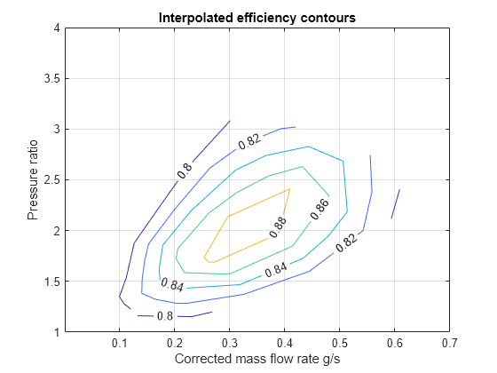
The contour plot shows that the interpolated efficiency contours match the source data. Additionally, the points are now in a format that the compressor block can use. If the generated compressor map has oversimplified contours or is missing key details, re-select your data using a denser mesh. You may need to select more points along each speed line, select points along estimated additional speed lines, or select more data points for each efficiency contour level.
Because this process interpolates data, there may be some precision loss. The only way to avoid this precision loss is to obtain the original raw test data used to generate the maps. Such data should contain a complete collection of corrected mass flow rates, pressure ratios, and efficiency values at a variety of operating conditions and speeds. This data, and the data used by the compressor block, is specified in the auxiliary coordinate system defined by the corrected speed, and the auxiliary coordinate β.
Implementing Compressor Maps in Simscape
In this example, the Compressor (G) block uses the workspace variables generated from the compressor map:
omega_TLUbeta_TLUpr_TLUmdot_TLUeta_TLU
For this model, the reference temperature and reference pressure are set to the inlet reservoir temperature and atmospheric pressure. Consequently, the corrected mass flow rate and corrected speed values are the same as the uncorrected values for the ideal angular velocity source, because the correction factor is equal to one. This model increases the pressure in a constant volume chamber by ramping up the compressor commanded speed.
 % Simulating model
sim('CompressorMap')

% Since Pressure and Temperature at A are at reference, mdot_A = mdot_corrected in grams/s
mdot_corrected = simlogCompressorMap.Compressor_G.mdot_A.series.values('g/s');

% Pressure Ratio
PR = simlogCompressorMap.Compressor_G.B.p.series.values ./ simlogCompressorMap.Compressor_G.A.p.series.values;

% The code below plots the compressor map using the same function as the
% Simscape block available by right clicking on the block and selecting
% Fluid > Plot Compressor Map
handle = getSimulinkBlockHandle('CompressorMap/Compressor (G)');
fluids.internal.mask.plotCompressorMap(handle)
hold on
% Plot operating line of compressor transient
plot(mdot_corrected, PR,'g','DisplayName','Operating Line')

The block compressor map matches the original source map. The interpolation process causes some error, but you can minimize the impact with good point selection practices.