Troubleshoot a Refrigeration Cycle

Working Models

The Model a Refrigeration Cycle with Varying Conditions example produces three models of increasing complexity:

The nominal design point targets a refrigerant mass flow rate of 0.03 kg/s.

Open the ModelADynamicRefrigerationCycleNominalOpenLoop model.

open_system('ModelADynamicRefrigerationCycleNominalOpenLoop');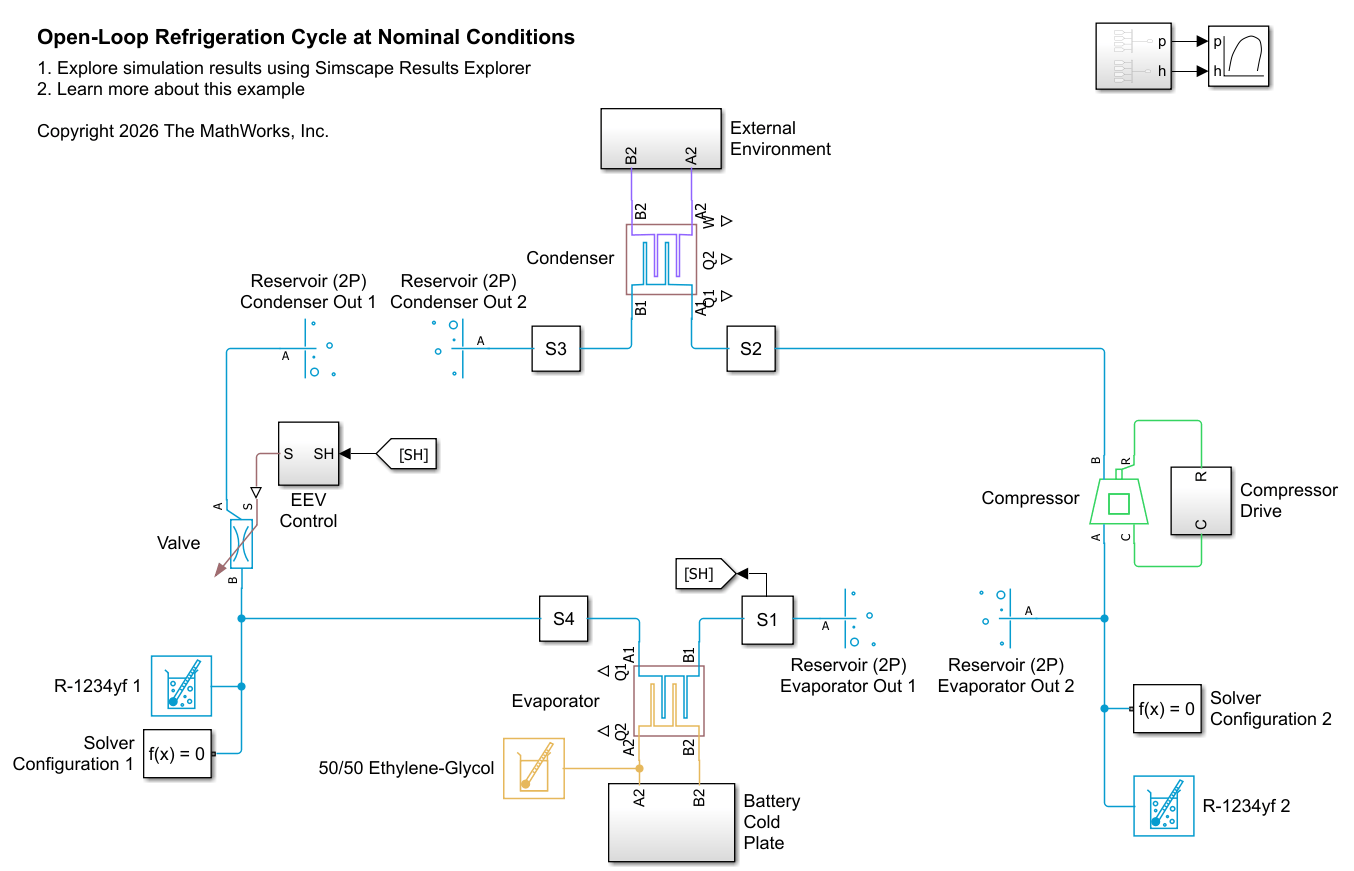

ModelADynamicRefrigerationCycleNominalOpenLoop is the open-loop harness model with reservoir boundary conditions. Use this model to validate component behavior, tune parameters, and debug initial conditions.

Open the ModelADynamicRefrigerationCycleNominalClosedLoop model.

open_system('ModelADynamicRefrigerationCycleNominalClosedLoop');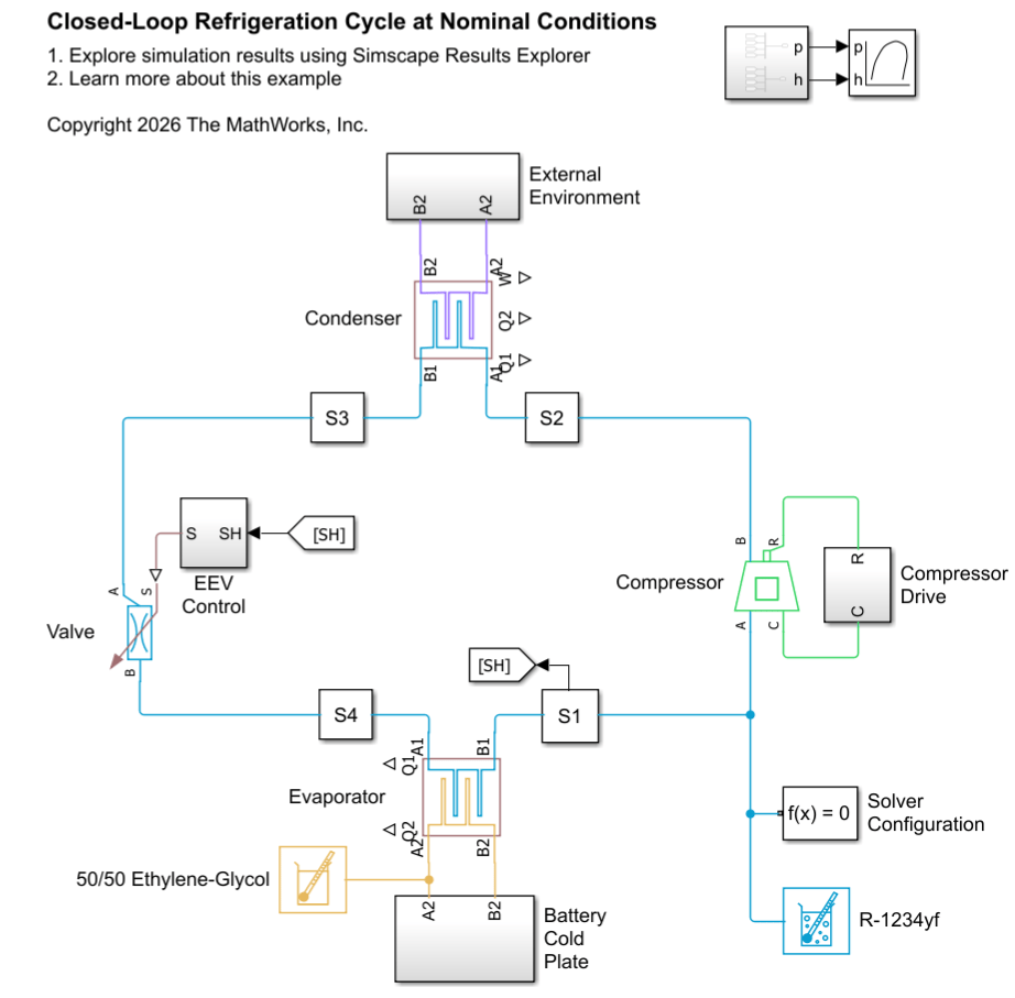

ModelADynamicRefrigerationCycleNominalClosedLoop is a closed-loop model at nominal conditions. This model validates that components work together in a closed circuit without controllers or accumulators.

Open ModelADynamicRefrigerationCycleVaryingClosedLoop.

open_system('ModelADynamicRefrigerationCycleVaryingClosedLoop');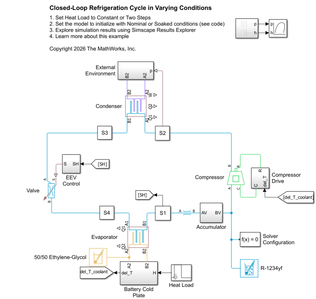

ModelADynamicRefrigerationCycleVaryingClosedLoop is the full refrigeration system with controllers and an accumulator. A coolant loop with a controller, expansion tank, and heat load models the load on the evaporator. This model handles varying heat loads and environmental conditions, and can initialize from a soaked state.

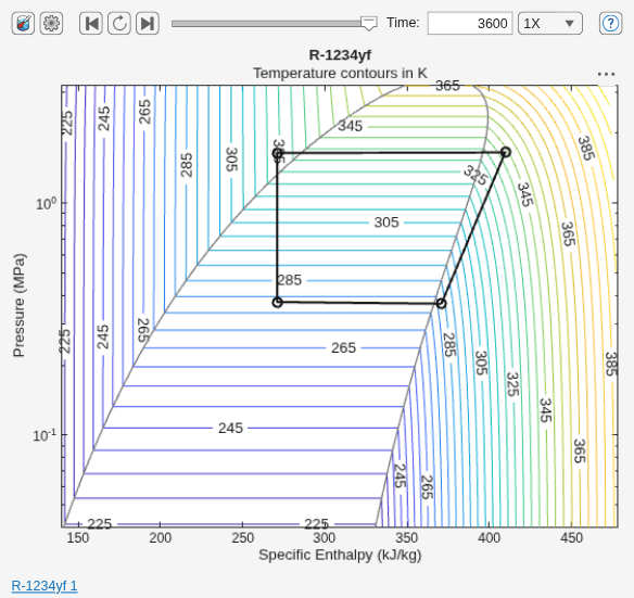
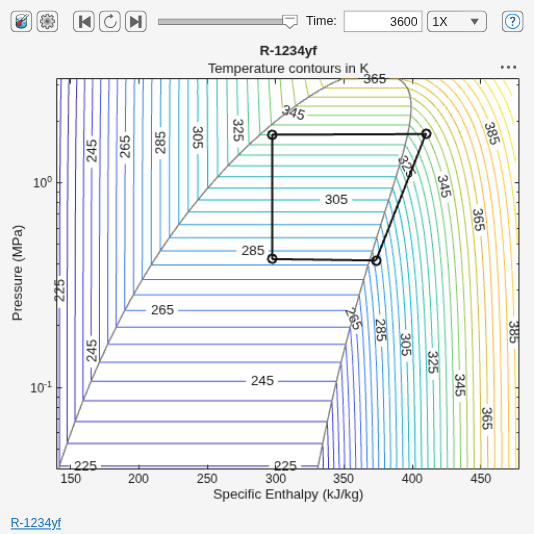
Simulate ModelADynamicRefrigerationCycleNominalOpenLoop and open the p-h diagram to see the nominal operating points.

sim('ModelADynamicRefrigerationCycleNominalOpenLoop');
open_system('ModelADynamicRefrigerationCycleNominalOpenLoop/P-H Diagram (2P)');

Issue 1: Error at Time = 0 (Nominal Conditions Start)

The first issue occurs in the ModelADynamicRefrigerationCycleNominalClosedLoop model. This issue can occur when you connect open-loop test harness models together to close the refrigeration loop.

Open the model and update parameters to contain the issue.

open_system('ModelADynamicRefrigerationCycleNominalClosedLoop');
IssueNumber = 1;
TroubleshootARefrigerationCycleInjectIssue;

Simulate the model and observe the issue.

try
    sim('ModelADynamicRefrigerationCycleNominalClosedLoop');
catch ME
    disp(ME.message);
    for i = 1:length(ME.cause)
        disp(ME.cause{i}.message);
    end
end

Warning: At time 0.000000e+00, one or more assertions are triggered. Fluid at port A must be fully vapor. The assertion comes from:
Block path: <a href="matlab:open_and_hilite_hyperlink ('ModelADynamicRefrigerationCycleNominalClosedLoop/Compressor','error')">ModelADynamicRefrigerationCycleNominalClosedLoop/Compressor</a>
Assert location: 
    o (location information is protected)

['ModelADynamicRefrigerationCycleNominalClosedLoop/Solver Configuration']: At time 0.000000e+00, one or more assertions are triggered. See causes for specific information.

Pressure at port B must be less than or equal to maximum valid pressure. The assertion comes from:
Block path: ModelADynamicRefrigerationCycleNominalClosedLoop/Compressor
Assert location: 
    o (location information is protected)

Pressure at port A1 must be less than or equal to maximum valid pressure. The assertion comes from:
Block path: ModelADynamicRefrigerationCycleNominalClosedLoop/Condenser
Assert location: 
    o (location information is protected)

The model errors shortly after initialization.

Identify the Cause

The error message references high pressure at the compressor outlet ports, and a warning states that fluid at the compressor inlet must be fully vapor. Both occur at t = 0, which indicates a bad initial state.

If a closed-loop model that initializes at nominal conditions errors at t = 0, revert to the open-loop model. Reservoir boundary conditions in the open-loop model prevent the failure, so the same bad initial conditions produce a visible transient instead of an error.

Open and simulate the open-loop model.

open_system('ModelADynamicRefrigerationCycleNominalOpenLoop');
sim('ModelADynamicRefrigerationCycleNominalOpenLoop');

Open the P-H Diagram (2P) block in the ModelADynamicRefrigerationCycleNominalOpenLoop model and set the Time to 0. Look for points that deviate from the nominal conditions:

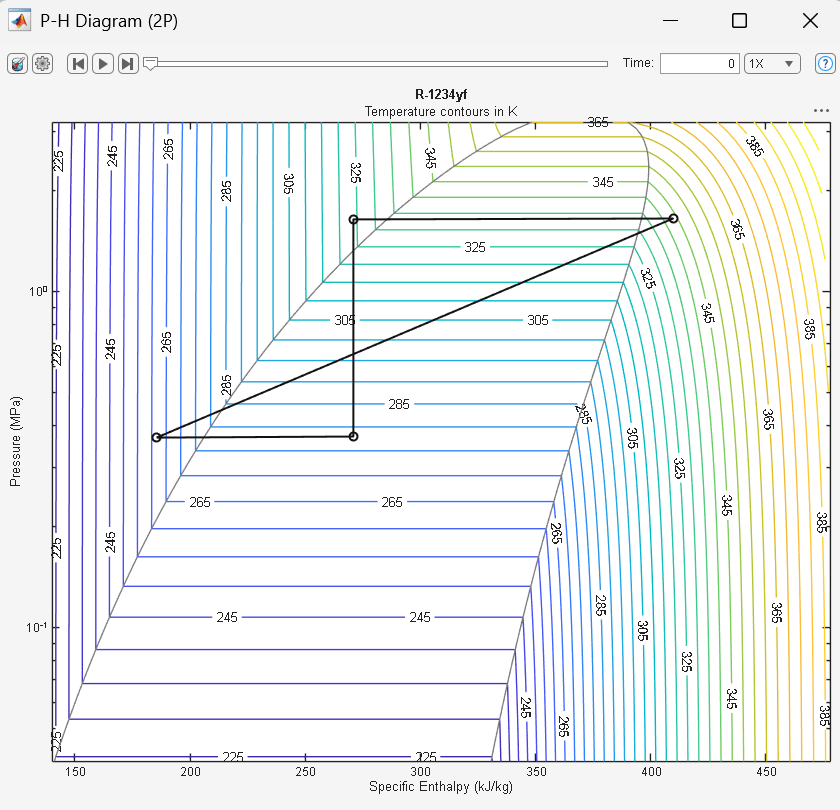
The specific enthalpy at the evaporator outlet in the open-loop model appears too low.

The observation aligns with diagnostic message from the closed-loop model. At 0.37 MPa, 185.5 kJ/kg is subcooled liquid for R-1234yf, not vapor, triggering the "must be fully vapor" warning in the compressor. In the closed-loop model, the compressor tries to compress liquid, generating extreme pressure that exceeds the property table bounds and triggers the "pressure must be less than maximum valid pressure" error.

Look at initial conditions specified in the evaporator block. The Initial two-phase fluid specific enthalpy parameter is set to the base workspace variable, RefrigerantEvaporatorInitialEnthalpy.

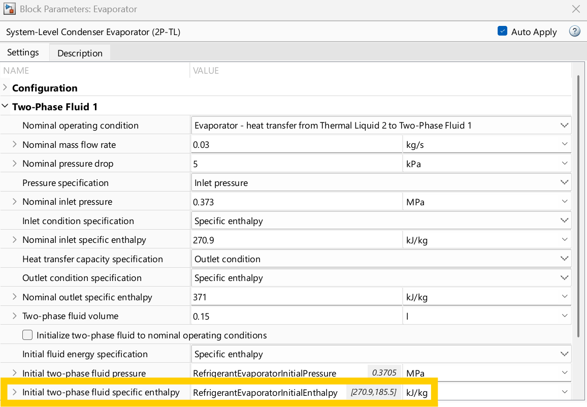
View the value of the base workspace variable:

disp(RefrigerantEvaporatorInitialEnthalpy);  % [kJ/kg]

  270.9000  185.5000

Diagnostic rule: If a state variable jumps rapidly from its initial value in the nominal open-loop model, the initial conditions do not match the intended nominal operating point. Adjust the initial conditions or nominal operating point characteristics.

Resolve the Issue

Correct the initial specific enthalpy setting in the evaporator to match the nominal operating point. The first element in the parameter corresponds to the inlet while the second element corresponds to the outlet:

RefrigerantEvaporatorInitialEnthalpy = [270.9 371]; % [kJ/kg]

Simulate the closed-loop model to confirm that changing the initial value resolved the issue.

sim('ModelADynamicRefrigerationCycleNominalClosedLoop');

Issue 2: Incorrect Steady-State P-H Points

Open the ModelADynamicRefrigerationCycleNominalClosedLoop model and inject a modeling issue into it.

open_system('ModelADynamicRefrigerationCycleNominalClosedLoop');
IssueNumber = 2;
TroubleshootARefrigerationCycleInjectIssue;

Simulate the model and open the p-h diagram.

sim('ModelADynamicRefrigerationCycleNominalClosedLoop');
open_system('ModelADynamicRefrigerationCycleNominalClosedLoop/P-H Diagram (2P)');

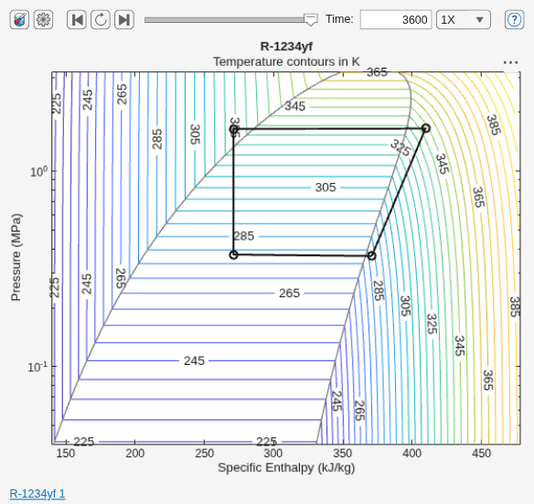
The model simulates without error, but the steady-state P‑H diagram no longer matches the nominal refrigeration cycle. The condenser does not subcool the refrigerant, and the operating pressures are slightly higher than intended.

Identify the Cause

When the condenser fails to achieve the desired subcooling, either:

For a refrigeration cycle operating at steady state, the condenser must reject all heat added by the evaporator and compressor.

The condenser heat transfer is:

where:

The compressor primarily determines refrigerant mass flow rate, while the condenser heat-transfer capability determines the outlet enthalpy.

Open the Results Explorer and inspect the refrigerant mass flow rate through the condenser.

sscexplore(simlog_NominalClosedLoop)

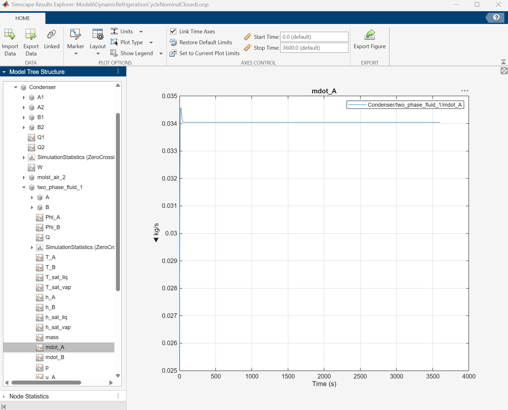
The refrigerant mass flow rate is close to the intended nominal value of 0.03 kg/s, indicating that the compressor is operating as expected. Therefore, the discrepancy originates from the condenser heat transfer rather than the refrigerant flow rate.

As described in Model a Refrigeration Cycle with Varying Conditions, the condenser was designed for the following nominal operating point:

The required nominal condenser heat transfer is therefore:

Q_nominal = 0.03 * (409.7 - 270.9)   % [kW]

Q_nominal = 
4.1640

When the condenser rejects less heat than this value, energy accumulates within the refrigeration cycle. The operating pressures and temperatures rise until the system reaches a different steady-state operating point, causing the P‑H diagram to drift from the intended nominal cycle.

The Nominal rate of heat transfer parameter in the Condenser block is set to the base workspace variable CondenserNominalQ, which is currently too low.

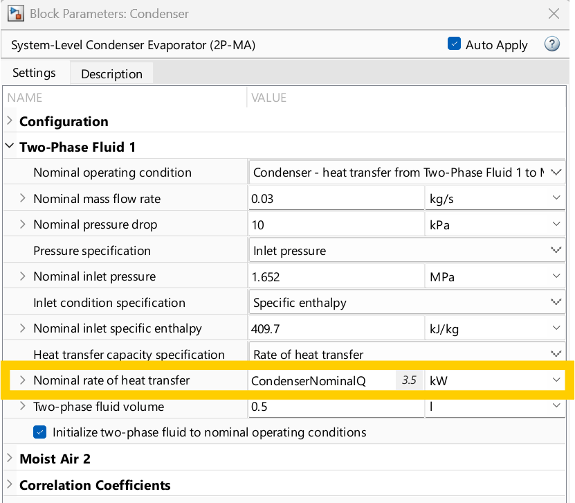
CondenserNominalQ

CondenserNominalQ = 
3.5000

Diagnostic rule: If the steady-state p‑h diagram does not match the intended nominal operating cycle, verify that each component satisfies the nominal energy balance. Use the open-loop harness models to identify the subsystem that deviates from its expected operating point.

Resolve the Issue

Set the condenser nominal heat transfer to balance the system:

CondenserNominalQ = Q_nominal; % [kW]

Simulate the closed-loop model to confirm that changing the initial value resolved the issue.

sim('ModelADynamicRefrigerationCycleNominalClosedLoop');
open_system('ModelADynamicRefrigerationCycleNominalClosedLoop/P-H Diagram (2P)');

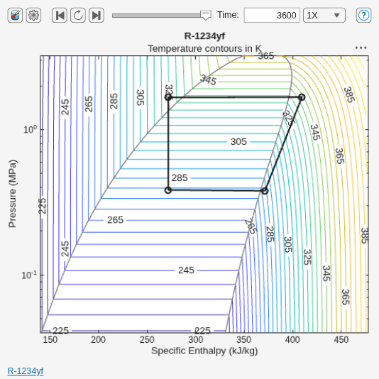
Issue 3: Error During a Load Transition

This issue occurs in the ModelADynamicRefrigerationCycleVaryingClosedLoop model when the heat load has a step change from 6 kW to 3 kW at t = 1800 s.

Open the model, set the heat load to varying, and inject the issue into the model.

open_system('ModelADynamicRefrigerationCycleVaryingClosedLoop');
set_param('ModelADynamicRefrigerationCycleVaryingClosedLoop/Heat Load', 'heatLoadType', 'Two Steps');
IssueNumber = 3;
TroubleshootARefrigerationCycleInjectIssue;

Simulate the model and observe the issue.

try
    open_system('ModelADynamicRefrigerationCycleVaryingClosedLoop/P-H Diagram (2P)');
    sim('ModelADynamicRefrigerationCycleVaryingClosedLoop');
catch ME
    disp(ME.message);
    for i = 1:length(ME.cause)
        disp(ME.cause{i}.message);
    end
end

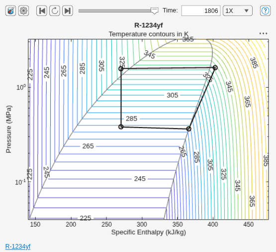
['ModelADynamicRefrigerationCycleVaryingClosedLoop/Solver Configuration']: At time 1805.659342, one or more assertions are triggered. See causes for specific information.

Fluid at port A must be fully vapor. The assertion comes from:
Block path: ModelADynamicRefrigerationCycleVaryingClosedLoop/Compressor
Assert location: 
    o (location information is protected)

Identify the Cause

The simulation errors shortly after the heat load drops from 6 kW to 3 kW. The diagnostic message indicates that refrigerant entering the compressor is no longer fully vapor.

The model operates normally at the initial steady-state operating point, but fails after the load change. This observation suggests that the nominal operating point and initial conditions are reasonable, but that the system cannot maintain valid operating conditions during the transient response.

To investigate, open the Results Explorer and examine signals that describe:

sscexplore(simlog_VaryingClosedLoop)

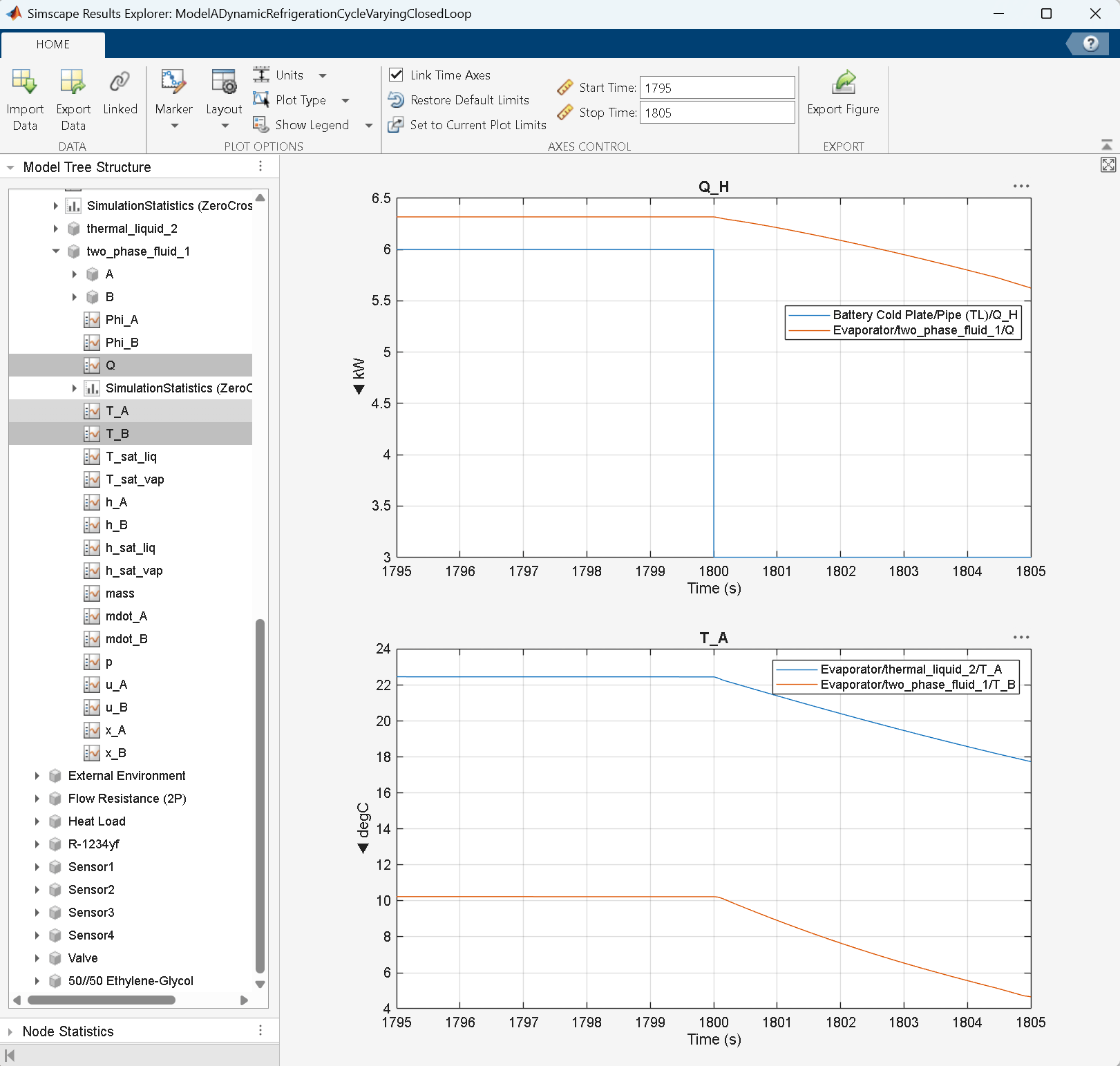
In this image of the Results Explorer, the Start Time is 1795 sec and the Stop Time to 1805 sec, to focus on the time when the error occurs. The simlog shows that the coolant temperature entering the evaporator (Evaporator/thermal_liquid/T_A) drops rapidly after the heat load step (Battery Cold plate/Pipe (TL)/Q_H). As a result, the heat transferred from the coolant to the refrigerant (Evaporator/two_phase_fluid_1/Q) also decreases quickly. As a result, the refrigerant temperature at the evaporator outlet drops quickly (Evaporator/two_phase_fluid_1/T_B).

Examine the responses of the controlled states.

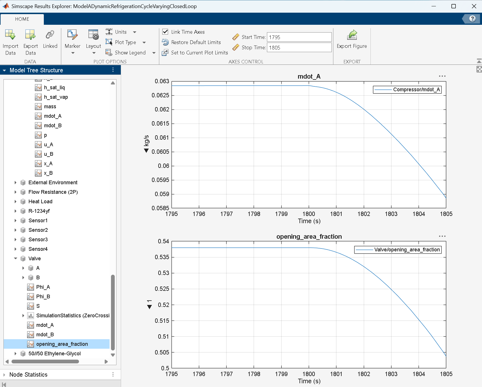
The controlled responses are much slower than the temperature changes. During the same time period, the compressor mass flow rate and electronic expansion valve (EEV) opening fraction change only slightly, so the refrigerant flow remains close to its pre-transition value.

Together, these observations reveal the source of the problem. The heat load decreases much faster than the refrigeration system can adapt. During the transition, the evaporator continues to receive nearly the same refrigerant flow even though much less heat is available to evaporate the refrigerant. As a result, the refrigerant leaves the evaporator at a lower vapor quality than intended. The evaporator outlet state moves toward the saturation boundary, and liquid refrigerant eventually reaches the compressor inlet, triggering the "must be fully vapor" diagnostic message.

Note that the sensor S1 in this model is positioned after the accumulator. If S1 were measured directly at the evaporator outlet, it would show vapor-liquid equilibrium (VLE) fluid during this transient, because the accumulator has not yet separated liquid from vapor.

The refrigeration cycle is correctly designed for both the initial and final operating points. The failure occurs because the system passes through temporary operating states during the transition. Transient operation therefore requires more design than selecting the correct steady-state operating points.

The root cause is a mismatch between the speed of the load change and the speed at which the refrigeration system can respond. Several design changes can improve transient robustness:

Resolve the Issue

Try option 1 first. CoolantVolumeFactor is a base workspace variable that scales the coolant volumes. Increase the coolant volumes by a factor of 10. Then try resimulating the system.

CoolantVolumeFactor = CoolantVolumeFactor * 10;
close_system('ModelADynamicRefrigerationCycleVaryingClosedLoop/P-H Diagram (2P)');
sim('ModelADynamicRefrigerationCycleVaryingClosedLoop');
disp('Successful simulation');

Successful simulation

Now try option 2 instead. Revert the coolant volume change. Then decrease the time constant of the EEV from 20 seconds to 5 seconds.

CoolantVolumeFactor = CoolantVolumeFactor / 10;
ValveTimeConstant = 5; % [s]
sim('ModelADynamicRefrigerationCycleVaryingClosedLoop');
disp('Successful simulation');

Successful simulation

Now try option 3. Revert the change of the valve time constant. Then add an accumulator at the evaporator outlet (by uncommenting the subsystem that's already included in the model).

ValveTimeConstant = 20; % [s]
set_param('ModelADynamicRefrigerationCycleVaryingClosedLoop/Accumulator', ...
    'Commented', 'off');
sim('ModelADynamicRefrigerationCycleVaryingClosedLoop');
disp('Successful simulation');

Successful simulation

Diagnostic rule: If a refrigeration model fails during a load transition, determine whether the refrigeration system can respond as quickly as the heat load changes. Compare the response times of:

A refrigeration system can operate correctly at both its initial and final steady-state operating points yet still fail while transitioning between them.

Restore the coolant volume sizes in the model.

CoolantVolumeFactor = 1;

Issue 4: P-H Diagram Drift (Soaked Start)

When a refrigeration system is off, all components eventually reach the ambient temperature and a common pressure. This condition is referred to as a soaked state.

Use the ModelADynamicRefrigerationCycleSoakedInit script to update the model settings so that it initializes in a soaked state. Then run the TroubleshootARefrigerationCycleInjectIssue script to inject a modeling issue.

open_system('ModelADynamicRefrigerationCycleVaryingClosedLoop');
set_param('ModelADynamicRefrigerationCycleVaryingClosedLoop/Heat Load', 'heatLoadType', 'Constant');
ModelADynamicRefrigerationCycleSoakedInit;
IssueNumber = 4;
TroubleshootARefrigerationCycleInjectIssue;

Simulate the model and observe the issue.

sim('ModelADynamicRefrigerationCycleVaryingClosedLoop');
open_system('ModelADynamicRefrigerationCycleVaryingClosedLoop/P-H Diagram (2P)');

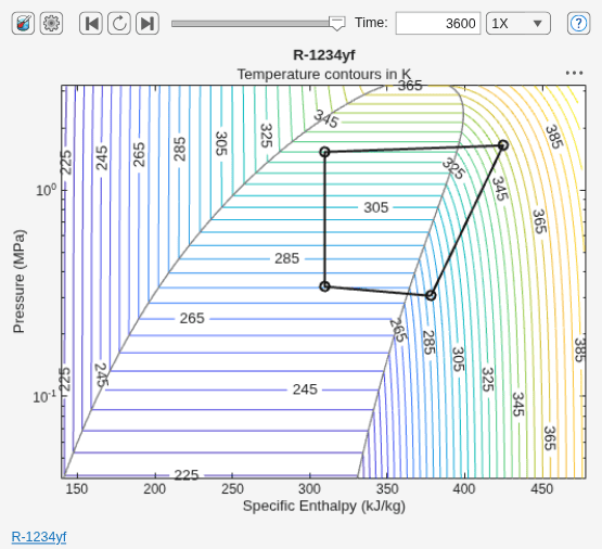
The model simulates successfully, but the p-h points have shifted to higher enthalpies than the nominal design points. The refrigeration cycle has not reached its intended steady-state operating point.

Identify the Cause

The p-h diagram shows two symptoms.

Open the Results Explorer to confirm. Even though the heat load and controller setpoints are at the nominal values:

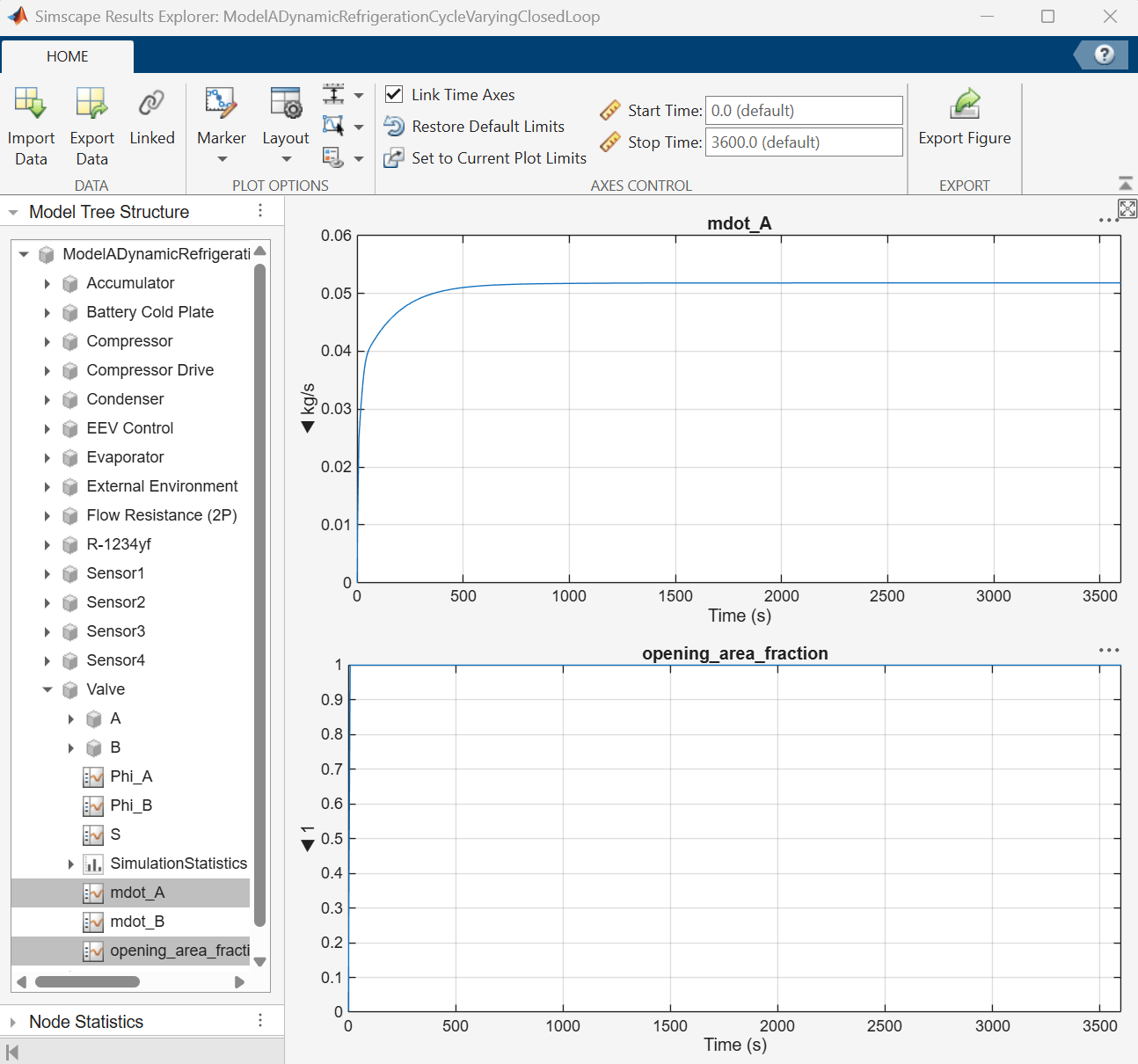
These observations are consistent with an undercharged refrigeration system. The evaporator is starved, so the superheat controller drives the expansion valve fully open. However, the refrigeration cycle does not contain enough refrigerant charge to reach the intended nominal operating point.

In a closed-loop model, refrigerant charge is determined by the initial states and component volumes. Once the simulation begins, refrigerant mass cannot enter or leave the loop, so the refrigerant charge remains constant throughout the simulation.

Calculate the refrigerant charge in the system. The ModelADynamicRefrigerationCycleNominalClosedLoop script obtains the refrigerant components' volume parameters and mass signals from the simlog. Then calculates the charge density.

ModelADynamicRefrigerationCycleCalculateRefrigerantMassVolume;
disp(TableMassVolume);

                   Volume (l)    Mass (kg)
                   __________    _________

    Evaporator        0.15       0.0027894
    Accumulator        0.5       0.0078534
    Condenser          0.5         0.07212
    Total             1.15        0.082762

The average charge density in the refrigeration loop is:

value(chargeDensity, 'kg/m^3')

ans = 
71.9673

The exact expected charge density depends on the type of refrigerant, volume distribution between high and low pressure side, and chosen nominal operating points. However, most systems typically have a charge density that is much higher than 72 kg/m^3.

Resolve the Issue

To initialize a refrigeration system from a soaked state, preserve the refrigerant charge required by the nominal operating point. Also, ensure that non-refrigerant parts of the system also initialize from an at-rest state.

Follow this fives-step process:

Step 1 - Determine the Refrigerant Charge at the Nominal Operating Point

The soaked-state refrigerant pressure depends on both temperature and refrigerant charge. Therefore, begin by determining the refrigerant charge that corresponds to the intended nominal operating point.

Use a script to adjust model parameters and variables to initialize the model at the nominal operating point. Then simulate the model:

ModelADynamicRefrigerationCycleNominalInit;
close_system('ModelADynamicRefrigerationCycleVaryingClosedLoop/P-H Diagram (2P)');
sim('ModelADynamicRefrigerationCycleVaryingClosedLoop');

Compute the total refrigeration loop volume, mass, and density at the nominal operating point. This model contains three blocks that hold refrigerant volume: the evaporator, accumulator, and condenser.

Use a script to obtain the volume of refrigerant in the components based on their volume parameters and the mass in each component at the nominal state based on the simlog. The ModelADynamicRefrigerationCycleCalculateRefrigerantMassVolume script also calculates charge density.

ModelADynamicRefrigerationCycleCalculateRefrigerantMassVolume;
disp(TableMassVolume);

                   Volume (l)    Mass (kg)
                   __________    _________

    Evaporator        0.15       0.0044311
    Accumulator        0.5        0.010003
    Condenser          0.5         0.19567
    Total             1.15         0.21011

The average charge density in the refrigeration loop at the nominal operating conditions is [kg/m^3]:

chargeDensity = RefrigerantTotalMass / RefrigerantTotalVolume;
value(chargeDensity, 'kg/m^3')

ans = 
182.7009

The nominal average charge density is much higher than the charge density of the model that initialized from a soaked state and converged to the wrong operating point. This confirms that the original soaked-state initialization did not preserve the refrigerant charge required by the nominal design.

Step 2 - Compute the Refrigerant States at the Soaked Temperature

When a refrigeration system is off, pressure equalizes throughout the loop. The soaked-state pressure is therefore determined by the refrigerant charge and ambient temperature rather than by the normal operating-point pressures.

The refrigerantChargeProperties function calculates fluid states based on the charge density and temperature.

[pressureSoaked, hSoaked, ~, uNormSoaked] = refrigerantChargeProperties( ...
    'ModelADynamicRefrigerationCycleVaryingClosedLoop/R-1234yf', chargeDensity, simscape.Value(Tatm, 'degC'));

The ModelADynamicRefrigerationCycleInitSoaked2P script applies the computed pressure, enthalpy, and internal energy to the evaporator, accumulator, and condenser in the ModelADynamicRefrigerationCycleVaryingClosedLoop model.

ModelADynamicRefrigerationCycleInitSoaked2P;

The script sets the accumulator to a saturated mixture (VLE) initial state and derives the initial liquid mass fraction from the normalized internal energy:

RefrigerantAccumulatorInitialLiquidMassFraction = 1 - value(uNormSoaked, '1');

Step 3 - Compute the Coolant States at the Soaked Temperature

Coolant mass in the thermal liquid loop must also be conserved. To determine the coolant pressure at the ambient temperature, this example uses a simplified harness model that starts from the nominal operating point and cools to the ambient temperature. If the expansion tank is sufficiently large relative to the coolant volume, coolant pressure remains nearly constant regardless of temperature. In that case, you can model a constant soaked pressure instead of simulating the coolant harness.

Open the coolant harness model.

open_system('ModelADynamicRefrigerationCycleCoolantLoopHarness');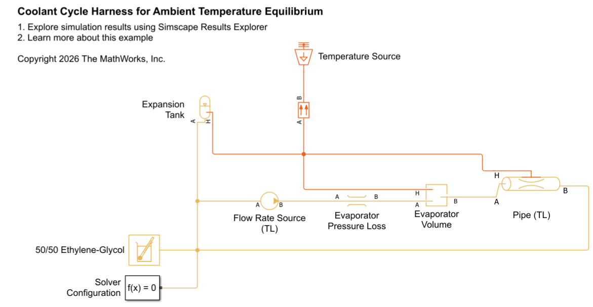

The harness contains only the components needed to represent the coolant mass and pressure losses. A Constant Volume Chamber (TL) and a Flow Resistance (TL) represent the Evaporator. The mass flow rate is set to 0 kg/s. A Temperature Source block set to the ambient temperature connects to the all the thermal ports of all blocks containing coolant volume. After the coolant reaches the ambient temperature, the pressure in the harness provides the soaked-state coolant pressure that can be used to initialize the full refrigeration model.

A similar approach could be used for the refrigerant loop. However, the refrigerantChargeProperties function provides a simpler way to determine soaked-state refrigerant conditions. The coolant loop is more difficult to treat analytically because the fluid volume changes with the state of the expansion tank.

Obtain the equilibrium pressure of the coolant from the last time step in the simlog.

sim(ModelADynamicRefrigerationCycleCoolantLoopHarness);
CoolantPressure = simlog_ModelADynamicRefrigerationCycleCoolantLoopHarness.Pipe_TL.p_I.series.values('MPa');
CoolantPressureSoaked = CoolantPressure(end);

The ModelADynamicRefrigerationCycleInitSoakedTL script applies the initial conditions to the coolant loop blocks in the ModelADynamicRefrigerationCycleVaryingClosedLoop model.

ModelADynamicRefrigerationCycleInitSoakedTL;

Step 4 - Update Initial Values of the Moist Air Components for the Soaked State

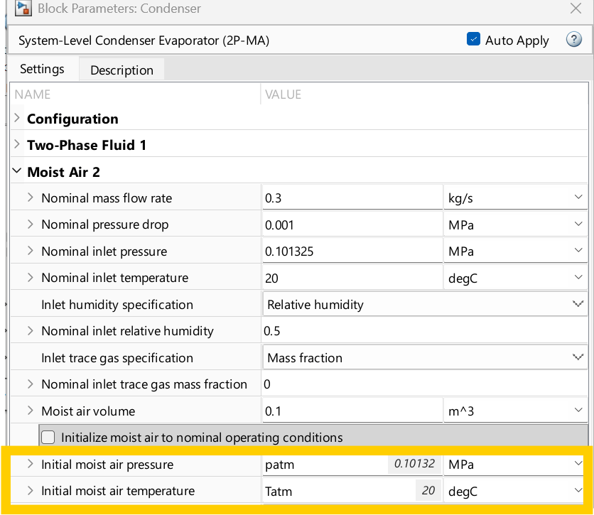
During a soaked condition, the condenser air is in equilibrium with the surrounding environment. Initializing the moist air side to nominal operating conditions would create an artificial temperature and pressure difference at startup. Uncheck the Initialize moist air to nominal operating conditions option in the Condenser. The parameters in the Condenser block are already configured to so that unchecking the option will initialize the Moist Air side of the condenser at atmospheric pressure and temperature.

In ModelADynamicRefrigerationCycleVaryingClosedLoop, the Moist Air Reservoirs already have atmospheric conditions, so they do not require any changes for the soaked initialization.

set_param('ModelADynamicRefrigerationCycleVaryingClosedLoop/Condenser', 'nominal_init_MA', 'false')

Step 5 - Update Initial Values of the Controllers for the Soaked State

The ModelADynamicRefrigerationCycleInitSoakedControllers script sets the PI controller integrators to small nonzero initial values. The controllers do not initialize at their nominal operating values because the system starts far from the nominal operating state. The nonzero values provide an initial control action during startup and help prevent the controllers from becoming stuck at zero output. Real systems often use dedicated startup control logic, but this example uses fixed initial controller values to keep the initialization procedure simple.

ModelADynamicRefrigerationCycleInitSoakedControllers;

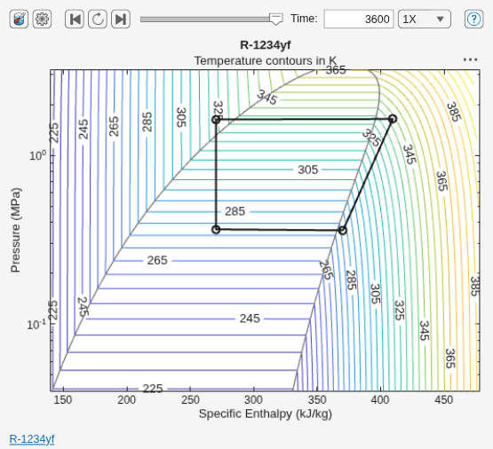
Simulate the model and observe the correct steady-state behavior after the soaked start.

sim('ModelADynamicRefrigerationCycleVaryingClosedLoop');
open_system('ModelADynamicRefrigerationCycleVaryingClosedLoop/P-H Diagram (2P)');

Diagnostic rule: When a closed-loop refrigeration model starts from a soaked state, initialize the refrigerant states so that they preserve the refrigerant charge required by the nominal operating point. If the soaked-state initial conditions establish the wrong refrigerant charge, the model can behave like an undercharged or overcharged refrigeration system and converge to an operating point different from the intended design.

Issue 5: Pressure Error (Soaked Start)

This issue occurs after changing refrigerant volumes in a refrigeration model that previously initialized correctly from a soaked state. After modifying the refrigerant volumes, the simulation fails shortly after startup.

First, open the model and initialize it from a soaked start at 20 degC ambient conditions.

IssueNumber = 5;
open_system('ModelADynamicRefrigerationCycleVaryingClosedLoop');
ModelADynamicRefrigerationCycleSoakedInit;
sim('ModelADynamicRefrigerationCycleVaryingClosedLoop');

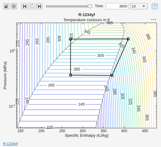
The model simulates successfully.

Now, redistribute volume in the refrigeration loop from the high-pressure side to the low-pressure side. Add 0.3 liters of refrigerant volume to the evaporator and subtract 0.3 liters from the condenser.

RefrigerantEvaporatorVolume = RefrigerantEvaporatorVolume + 0.3; % [l]
RefrigerantCondenserVolume  = RefrigerantCondenserVolume  - 0.3; % [l]

The system has the same total refrigerant volume as before, but now a larger fraction of the volume in on the low-pressure side and a smaller fraction is on the high-pressure side.

Simulate the model.

open_system('ModelADynamicRefrigerationCycleVaryingClosedLoop/P-H Diagram (2P)');
try
    sim('ModelADynamicRefrigerationCycleVaryingClosedLoop');
catch ME
    disp(ME.cause{1}.message);
end

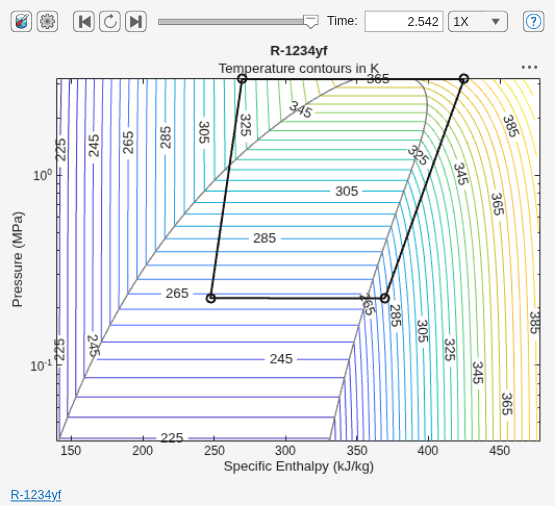
Pressure at port B must be less than or equal to maximum valid pressure. The assertion comes from:
Block path: ModelADynamicRefrigerationCycleVaryingClosedLoop/Compressor
Assert location: 
    o (location information is protected)

The simulation errors at around 2.5 seconds with a maximum pressure violation in the condenser.

Identify the Cause

Issue 4 showed that soaked-state initialization must preserve the refrigerant charge required by the nominal operating point.

Increasing the evaporator volume and decreasing the condenser volume changes the volume distribution between the low-pressure side and high-pressure side of the refrigeration cycle.

Refrigerant on the high-pressure side is much denser than refrigerant on the low-pressure side. As a result, moving refrigerant volume from the condenser to the evaporator changes the refrigerant charge required to reach the nominal operating point.

Although the total refrigerant volume remains unchanged, the average charge density at the nominal operating point changes.

The original soaked-state initialization no longer matches the updated model configuration. During startup, the refrigeration cycle contains too much refrigerant charge for the new volume distribution, causing the condenser pressure to exceed its valid operating range.

For reference, view the current average charge density in the system.

value(chargeDensity, 'kg/m^3')

ans = 
182.6957

Resolve the Issue

Recalculate the soaked-state initialization for the updated refrigerant volume distribution.

Use the same five-step process described previously for resolving Issue 4:

The following script performs these steps:

ModelADynamicRefrigerationCycleSoakedInit;

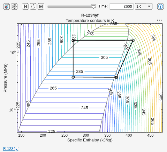
Check the updated charge density.

value(chargeDensity, 'kg/m^3')

ans = 
88.4897

The updated charge density for the redistributed volumes is much lower than the previous charge density.

Simulate with corrected initial conditions:

sim('ModelADynamicRefrigerationCycleVaryingClosedLoop');
open_system('ModelADynamicRefrigerationCycleVaryingClosedLoop/P-H Diagram (2P)');

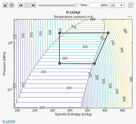
The system starts up correctly and reaches the expected operating points.

Diagnostic rule: When a closed-loop refrigeration model starts from a soaked state, initialize the refrigerant states so that they preserve the refrigerant charge required by the nominal operating point. Changing refrigerant component volumes or nominal p-h states changes the nominal charge density, so you need to recalculate refrigerant states in a soaked start.

Key Takeaways