Parameterize an M-Way N-Position Valve

To model a valve configuration that does not match a predefined Simscape™ Fluids™ directional valve block, you can use the M-Way N-Position Directional Valve (IL) block. This block models a directional valve with a custom configuration of ports, spool positions, and orifices. The block accepts up to ten ports, ten spool positions, and 20 orifices. In this example, you parameterize the block using a hypothetical manufacturer data sheet.

Configure the Valve Geometry

When parameterizing the M-Way N-Position Valve (IL) block, the best practice is to first match the block geometry to a valve schematic. Consider this valve schematic.

4-way 4-position valve schematic

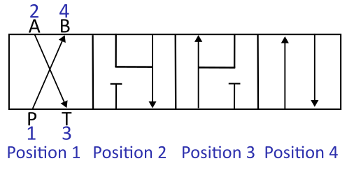
Flow Path on Data Sheet	Corresponding Block Orifice
P → B	Orifice 1
A → T	Orifice 2
P → A	Orifice 3
B → T	Orifice 4

Add the M-Way N-Position Valve (IL) block to your model. To configure the block parameters to match the valve geometry, use the information from the data sheet:

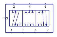
Assign each port in the valve schematic a number that corresponds to the M-Way N-Position Valve (IL) port names. Valve schematics typically label valve ports as A, B, P, and T, while the port names for the M-Way N-Position Valve (IL) block are numbers that start at the lower-left port and alternate sides as they increase. In this schematic, the numbers correspond to the block ports.
Identify the values for the Number of ports, Number of spool positions, and Number of orifices parameters. Because this valve is a four-way, four-position valve, and there are four possible flow paths through the valve, the value for each of these parameters is 4.
Identify the orifices and configure the connected ports. In this schematic, ports 1 and 4, 2 and 3, 1 and 2, and 3 and 4 are connected. The order of the ports dictates the direction the arrows point, but the flow can go in either direction. Set:
- Ports connected by orifice 1 to [1,4]
- Ports connected by orifice 2 to [2,3]
- Ports connected by orifice 3 to [1,2]
- Ports connected by orifice 4 to [4,3]
Configure the spool positions where each orifice is open. Each panel in the schematic corresponds to one spool position. For this schematic, set:
- Spool position indices where orifice 1 is open to [1,3]
- Spool position indices where orifice 2 is open to [1,2]
- Spool position indices where orifice 3 is open to [3 4]
- Spool position indices where orifice 4 is open to [2,4]

Note

The block always adds additional ports on alternating sides of the block. To model a valve with more than one additional port on a side, add an extra port unconnected to any orifice. For example, to model a valve with 4 ports on one side and 2 on the other, set Number of ports to 7. In this configuration, port 2 is unused.

Block diagram parameterized to be have 4 active ports on one side and 2 on the other

Determine Flow Rate and Pressure Drop Parameters

After configuring the valve geometry, you can use the Graph Importer tool to help parameterize the block. Consider a data sheet with these flow rate–pressure drop curves.

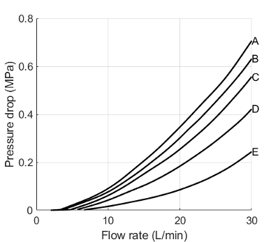
Flow rate–pressure differential curves

Use the flow rate–pressure differential curves to configure the block flow rate and pressure drop parameters:

Identify the data for your valve. This table shows the flow paths as they are typically labeled on a data sheet, the corresponding orifice for the block, and the flow rate–pressure drop curve for that orifice.
Flow Path on Data Sheet Corresponding Block Orifice Flow Rate—Pressure Drop Curve
P → B Orifice 1 A
A → T Orifice 2 A
P → A Orifice 3 C
B → T Orifice 4 D
Use the Graph Importer app to import the data for curves A, C, and D. For more information on how to use this app, see Graph Importer.

Flow Path on Data Sheet	Corresponding Block Orifice	Flow Rate—Pressure Drop Curve
P → B	Orifice 1	A
A → T	Orifice 2	A
P → A	Orifice 3	C
B → T	Orifice 4	D

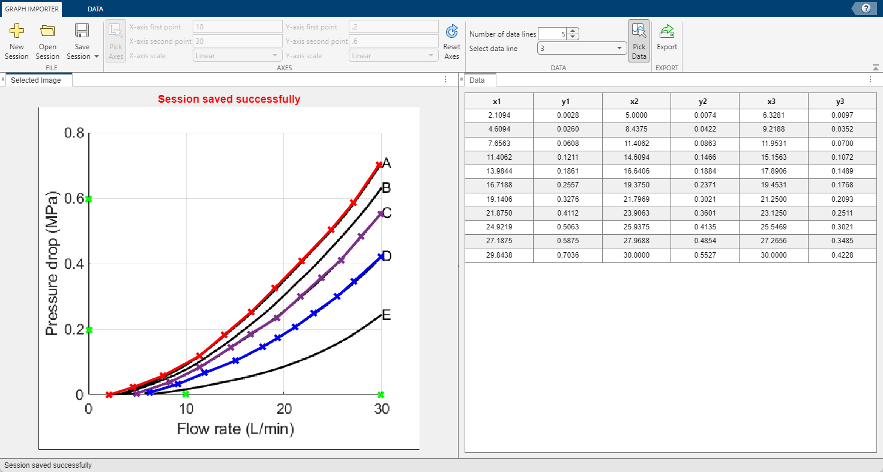
After you select the data, export it and save it in your working directory. Load the file into the MATLAB^® workspace. The columns of the resulting tableData matrix contain the pressure drop and flow rate data for the orifices.

load mway_valve
% Data for orifices 1 and 2
orifice12_flowrate=tableData(:,1);
orifice12_pressuredrop=tableData(:,2);
% Data for orifice 3
orifice3_flowrate=tableData(:,3);
orifice3_pressuredrop=tableData(:,4);
% Data for orifice 4
orifice4_flowrate=tableData(:,5);
orifice4_pressuredrop=tableData(:,6);

Because this data sheet provides different flow rate–pressure differential curves for each orifice, set the Area characteristics parameter of the M-Way N-Position Directional Valve (IL) block to Different for each flow path and the Orifice Parameterization parameter to Tabulated data - Volumetric flow rate vs. pressure drop (linear with spool travel). If your data sheet differential curves are in terms of area vs. spool travel, set the Orifice Parameterization parameter to Tabulated data - Area vs. spool travel.
Set the Pressure drop of orifice and Fully open volumetric flow rate vector of orifice parameters to the corresponding variables for each orifice. Set the units for each Fully open volumetric flow rate vector of orifice parameter to lpm.

Determine Spool Travel Parameters and Confirm Block Behavior

Most data sheets do not explicitly contain information on spool travel lengths. However, the sheet may provide a cutaway image of the valve that you can use to estimate distances. For many valves, you can approximate the spool travel parameters based on the assumption that the distance between each discrete spool position and the difference between each spool travel position index is 1 mm. You can use these assumed values to set the Spool travel for which orifice remains fully open and Spool travel at each position index parameters, respectively. You can also assume that the value of the Spool travel for which orifice transitions between open and closed parameter is on the order of 0.25 mm.

Use the valve characteristic plot to visualize the volumetric flow rate at a set pressure drop across the spool positions and confirm that the plot reflects the intended characteristics.

Generate the characteristic plot of the valve. Right-click the block and select Fluids > Plot Valve Characteristics. This image uses the pressure drop and flow rate data from the previous section and the following settings:
- Spool travel at each position index to [0,1,2,3] mm
- Spool travel for which orifice remains fully open to 1 mm for all orifices
- Spool travel for which orifice transitions between open and closed to 0.25 mm for all orifices
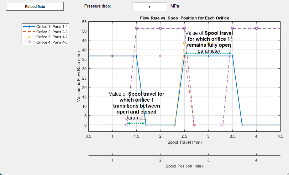
Confirm that the spool travel matches the values you specified in the parameters. For example, the characteristic plot shows that orifice 1 remains open for 1 mm of spool travel and takes 0.25 mm of spool travel to close, which matches the values specified in the Spool travel for which orifice 1 remains fully open and Spool travel for which orifice 1 transitions between open and closed parameters.
Confirm that each orifice is in the intended position at each spool position. For example, the Spool position indices where orifice 1 is open parameter specifies that orifice 1 should be open in spool positions 1 and 3, which the characteristic plot reflects.
Validate the volumetric flow rate behavior. The flow rate changes linearly in the characteristic plot because when Orifice Parameterization is Tabulated data - Volumetric flow rate vs. pressure drop (linear with spool travel), the block assumes that the volumetric flow rate is linear with respect to spool travel.
The flow rate–pressure differential curves from the data sheet show that orifice 4 has a lower pressure drop for a given flow rate value compared to the other orifices. Conversely, for a fixed pressure drop, orifice 4 has the highest flow rate. The characteristic plot reflects that behavior, and shows that at a fixed pressure drop, orifice 4 has the highest volumetric flow rate when open.
You can also click the appropriate orifice on the legend to select which lines are visible. For each orifice, you can adjust the value in the Pressure drop box to verify that the maximum flow rate corresponds to the pressure drop and flow rate data in the data sheet curve.

To further validate your parameterized block, create a test harness model for the block and compare the results to data from a physical system. For more information on building a test harness model for a directional control valve, see 4-Way 3-Position Valve Parameterization.