Estimate Nonlinear ARX Model Using Dynamic System Learner App
R2026bThe Dynamic System Learner app trains models for time series modeling. This topic explains how to train a nonlinear autoregressive with exogenous input (ARX) model using the Dynamic System Learner app.
Using this app, you can:
Import and visualize time series data.
Specify data preprocessing options such as splitting the data into training and validation sets.
Select the nonlinear ARX model type from a list of predefined models. You can identify nonlinear ARX models by using nonlinear identification algorithms in the System Identification Toolbox™ software.
Configure the nonlinear ARX model by specifying model structure and training options.
Visualize training metrics and select a trained model from a list of candidate models.
Compare the predictions of your trained model to the measured training and validation data sets.
Export the trained model and generate MATLAB® code to help you predict on new data.
For more information on the app, see Dynamic System Learner.
Open App and Import Data
To open the Dynamic System Learner app, at the MATLAB command prompt, enter dynamicSystemLearner. You can also
open the app by selecting Dynamic System Learner from the
MATLAB
Apps gallery.
To import data from the MATLAB workspace into the app, on the toolstrip, click New > Numeric or timetable or New > iddata. The Import Data dialog box opens. For information on the available options in the Import Data dialog box, see Open App and Import Data.
Preview Imported Data
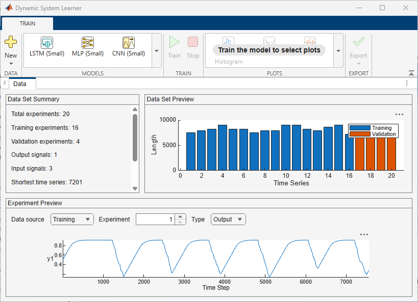
The app displays the data you import in the Data tab. In this tab:
A summary of the imported data appears in the Data Set Summary section.
You can preview individual experiments in the Experiment Preview section.
If the imported data includes multiple experiments, you can also view a plot of the experiments and their corresponding time steps in the Data Set Preview section.
Configure Nonlinear ARX Model Structure and Training Options
Model Structure Configuration
To configure the nonlinear ARX model structure you want to train, in the app, select Nonlinear ARX Model from the Models gallery. The Model tab opens in the app along with its Summary tab. For more information on nonlinear ARX models, see What Are Nonlinear ARX Models?
In the Summary tab, specify the structure of the model by using these options under Model Structure:
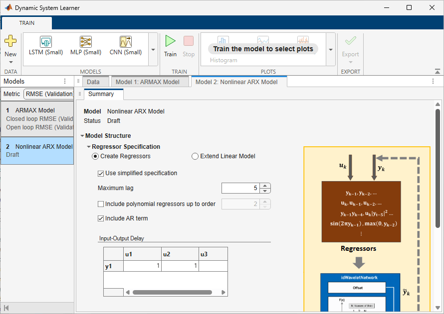
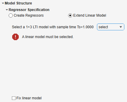
Regressor Specification — To specify regressors, select either Create Regressors or Extend Linear Model. Each choice gives you a different set of options to configure.
To simplify regressor specification, select Create Regressors and then select Use simplified specification. Configure the options that appear.
Maximum lag — Specify the maximum number of past lags in the imported output and input values that are used to predict the current model output, as a positive scalar. The maximum lag you specify must be greater than the values in the Input-Output Delay matrix (whose default values are one).
Include polynomial regressors up to order — Select this option to include polynomial regressors using all input and output variables with lags in each variable from
1to the Maximum lag value. Specify the order of the polynomial, as a scalar integer greater than1.Include AR term — Select this option to include the autoregressive term in the model structure.
Input-Output Delay — This option appears only when you import both outputs and inputs. Use this option to specify the input-output delay, also called the transport delay, as an Ny-by-Nu matrix of nonnegative integers. Here, Ny is the number of outputs and Nu is the number of inputs. The values you specify in the Input-Output Delay matrix must be less than the Maximum lag value.
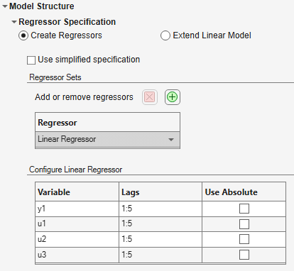
To specify regressors explicitly, select Create Regressors and then clear Use simplified specification. Under Regressor Sets, in the table, you can select
Linear Regressor,Polynomial Regressor,Periodic Regressor, orCustom Regressor. Each choice gives you corresponding options to configure. You can also add or delete regressors from the table.Configure Linear Regressor — This section appears only when you select
Linear Regressor. For each variable, in the Lags column, specify the regressor lags as a row vector of nonnegative integers. To use the absolute value of a regressor variable instead of the signed value, select the box in the Use Absolute column. For more information on linear regressors, seelinearRegressor.Configure Polynomial Regressor — This section appears only when you select
Polynomial Regressor. Specify the order of the polynomial, as a scalar integer greater than1. For each variable, in the Lags column, specify the regressor lags as a row vector of nonnegative integers. To use the absolute value of a regressor variable instead of the signed value, select the box in the Use Absolute column. To specify multiple variables in regressor formulas, select Mix Variables. To use different lags in regressor formulas, select Mix Lags. For more information on polynomial regressors, seepolynomialRegressor.Configure Periodic Regressor — This section appears only when you select
Periodic Regressor. For each variable, in the Lags column, specify the regressor lags as a row vector of nonnegative integers. To use the absolute value of a regressor variable instead of the signed value, select the box in the Use Absolute column. To apply the same frequency multiplier to all the regressors, specify Multiplier as a scalar. To specify the number of terms to use for each lagged variable, specify Number of terms as a scalar positive integer. To generate sine and cosine regressors, select Use sine and Use cosine, respectively. For more information on periodic regressors, seeperiodicRegressor.Configure Custom Regressor — This section appears only when you select
Custom Regressor. In Custom formula, specify the custom function that transforms a set of delayed variables into a numeric scalar output. Specify this function as an expression using the variables in the table below. For each variable, in the Lags column, specify the regressor lags as a row vector of nonnegative integers. For more information on custom regressors, seecustomRegressor.
To specify the model orders and the initial values of the model linear coefficients using an existing linear model, select Extend Linear Model. From the MATLAB workspace, select an LTI model with the same number of inputs and outputs and the same sample time as the data you imported. To fix the linear portion of the nonlinear ARX model during estimation so that it remains identical to the selected linear model, select Fix linear model.
Output Functions — Select the output function that maps the regressors of the nonlinear ARX model into the model output as
Linear,Sigmoid Network,Wavelet Network, orCustom Network.For
Sigmoid Network,Wavelet Network, andCustom Network, specify Number of units as a positive integer. This value determines the number of sigmoid functions, wavelets, and custom unit functions, respectively. ForWavelet Network, you can choose to automatically select the number of units.For
Custom Network, specify Custom function name as a function handle.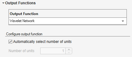
For information on configuring nonlinear ARX models programmatically, see idnlarx.
Training Options Configuration
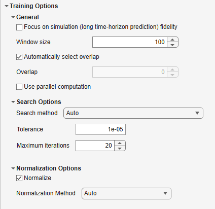
To control how the app trains the model, specify these options under Training Options in the Summary tab:
General
Focus on simulation (long time-horizon prediction) fidelity — Select this option to minimize the simulation error between measured and simulated outputs during estimation. The estimation focuses on making a good fit for simulation of model response with the current inputs. This option is available only when you import both outputs and inputs.
Window size — Specify the number of samples in each frame or batch when segmenting data for model training, as a positive integer.
Automatically select overlap — Select this option to automatically select the size of the overlap to be equal to the maximum delay across all model regressors.
Overlap — Specify the number of samples in the overlap between successive frames when segmenting data for model training, as an integer. A negative integer indicates that certain data samples are skipped when creating the data frames. You can specify this option only if you do not select Automatically select overlap.
Use parallel computation — Select this option to enable parallel computing for model training. Use parallel computing to simultaneously train multiple candidate models based on the model structure you specify.
Search Options
Search method — Specify the numerical search method to use for iterative parameter estimation as
Auto,Gauss-Newton (gn),Adaptive Gauss-Newton (gna),Levenberg-Marquardt (lm),Gradient Descent (grad),Trust-region Reflective Newton (lsqnonlin),Pattern Search (patternsearch), orConstrained Nonlinear Optimization (fmincon). Each method has associated options that you can configure.Search Method Configuration Option Value AutoGauss-Newton (gn)Adaptive Gauss-Newton (gna)Levenberg-Marquardt (lm)Gradient Descent (grad)
Tolerance Positive scalar Maximum iterations Positive integer Trust-region Reflective Newton (lsqnonlin)Function Tolerance Positive scalar Step Tolerance Positive scalar Maximum iterations Positive integer Pattern Search (patternsearch)Use parallel computation Algorithm ClassicNonuniform Pattern SearchNonuniform Pattern Search (GPS)Nonuniform Pattern Search (MADS)
Function Tolerance Positive scalar Step Tolerance Positive scalar Automatically choose max iterations Constrained Nonlinear Optimization (fmincon)Algorithm Sequential Quadratic ProgrammingInterior PointTrust-regionActive Set
Function Tolerance Positive scalar Step Tolerance Positive scalar Maximum iterations Positive integer For more information on the search methods and options, see
SearchMethodandSearchOptions.
Normalization Options
Normalize — Select this option to normalize estimation data using the method specified in Normalization Method.
Normalization Method — Specify the method to use to normalize estimation data as
Auto,Center,Z-Score,Norm,Scale,Range, orMedian Interquartile Range. Some methods have an associated option that you can configure.Normalization Method Configuration Option Value CenterCentering method MeanMedian
Z-ScoreZ-Score method Standard DeviationRobust
NormNorm value Positive integer ScaleScale method Standard DeviationMedian Absolute DeviationInterquartile RangeFirst Element
RangeRange Two nonnegative scalars For more information about the normalization methods and options, see
NormalizationOptions.
Train Nonlinear ARX Model
To train the configured nonlinear ARX model, on the toolstrip, click Train. The Model Selector tab
opens next to the Summary tab. The Training Information section appears with the statement: Trying
various model structures and fitting algorithms….
Model Selection
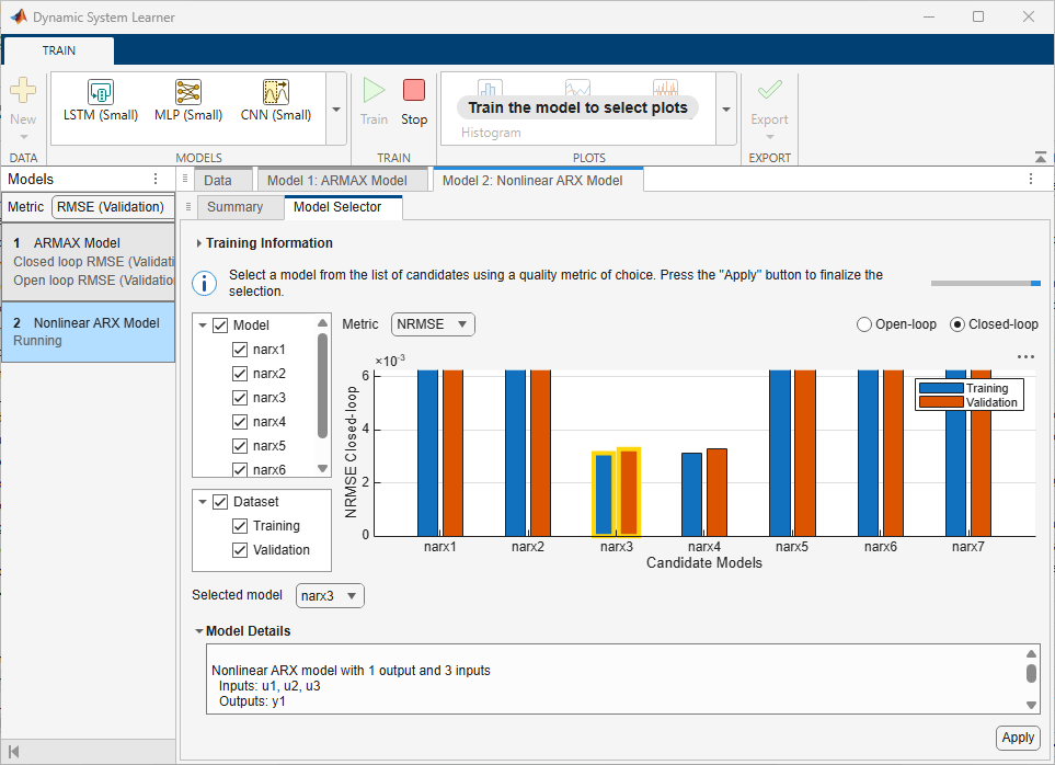
After model training, the app produces between one and seven candidate models. A plot
displaying the candidate models and their respective metric values appears on the
Model Selector tab. At the top of the plot, in the
Metric menu, choose the quality metric that you want
the plot to display. The available metrics are RMSE,
NRMSE, MAE,
AIC, and BIC. For more information
on the metrics, see the Model Selection section in Estimate ARMAX Model Using Dynamic
System Learner App.
To the left of the plot, you can choose which models to display. You can choose to
display the Training dataset,
Validation dataset, or both.
If you choose RMSE, NRMSE, or
MAE as the metric to display, then you can select Open-loop or Closed-loop at the
top right of the plot to display the respective plots.
| Metric Generation Setting | Description |
|---|---|
| Open-loop | Selecting the metric setting as Open-loop is
equivalent to specifying the prediction horizon input argument for the |
| Closed-loop | Selecting the metric setting as Closed-loop is
equivalent to specifying the prediction horizon input argument for the |
The plot automatically highlights the model with the lowest NRMSE value on training data in the closed-loop metric setting. You can also see that the app selects this model in the Select model list and displays its information in the Model Details section. You can select a different model by clicking the model in the plot or selecting it in the Select model list.
The qualities of the candidate models change based on the metric type and metric setting you choose. A candidate model with a lower value for your chosen metric is better. When selecting a model, you can also weigh the value of the chosen metric against the complexity of the model.
If the app produces more than one candidate model, then select a model and click Apply to complete the training process with that model. If the app produces only one candidate model, then it automatically selects that model and completes the training process. In this case, the app does not wait for you to click Apply.
Analyze Performance Using Plots
To analyze the performance of your model, you can generate these plots for either the training or validation data: Predict, RMSE Histogram, Residuals, and Residual Histogram. For more information on these plots, see Predict Values for Data, Plot RMSE Histogram, Plot Residuals, and Plot Residual Histogram.
Export Trained Model
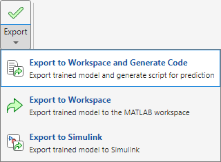
To export the trained model and the training statistics to the MATLAB workspace and generate a live script for predicting on new data, on the
toolstrip, click Export. The app exports a structure that
contains an idnlarx model and generates a live script that
contains code for preparing and predicting values for new data.
To only export the trained model to the MATLAB workspace and not generate code, click Export > Export
to Workspace. The app exports a structure that contains an idnlarx model.
To export the trained model to Simulink® as an Nonlinear ARX Model block, click Export > Export to Simulink. The Export to Simulink dialog box opens. In this dialog box, you can choose to export the trained model as one of these model types:
Simulation model — The generated Idmodel block has only one input port for injecting input signals.
Finite-horizon prediction model — The generated Idmodel block has two input ports, one for injecting input signals and one for injecting the measured output values. In the Export to Simulink dialog box, you specify Horizon (number of steps) as a positive integer.
You can also specify the folder in which the app will save the Simulink model. By default, the app saves the model in the current working folder.