Use LSTM Network for Linear System Identification
R2026bThis example shows how to use long short-term memory (LSTM) neural networks to estimate a linear system and compares this approach to transfer function estimation.
In this example, you investigate the ability of an LSTM network to capture the underlying dynamics of a modeled system. To do this, you train an LSTM network on the input and output signal from a linear transfer function, and measure the accuracy of the network response to a step change.
Transfer Function
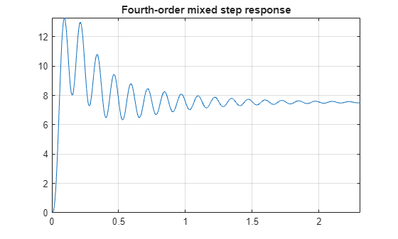
This example uses a fourth-order transfer function with mixed fast and slow dynamics and moderate damping. The moderate damping causes the system dynamics to damp out over a longer time horizon and shows the ability of an LSTM network to capture the mixed dynamics without some of the important response dynamics damping out. Construct the transfer function by specifying the poles and zeros of the system.
fourthOrderMdl = zpk(-4,[-9+5i;-9-5i;-2+50i;-2-50i],5e5);
[stepResponse,stepTime] = step(fourthOrderMdl);
Plot the step response of the transfer function.
plot(stepTime,stepResponse)
grid on
axis tight
title('Fourth-order mixed step response')
The Bode plot shows the bandwidth of the system, which is measured as the first frequency where the gain drops below 70.8%, or around 3 dB, of its DC value.
bodeplot(fourthOrderMdl)
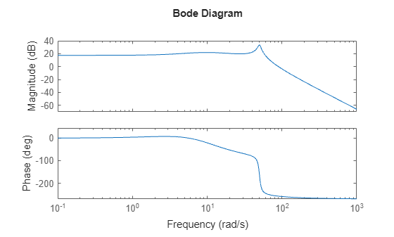
fb = bandwidth(fourthOrderMdl)
fb =
62.8858
Generate Training Data
Construct a data set of input and output signals that you can use to train an LSTM network. For the input, generate a random Gaussian signal. Simulate the response of the transfer function fourthOrderMdl to this input to obtain the output signal.
Gaussian Noise Data
Specify properties for the random Gaussian noise training signal.
rng default
signalType = 'rgs'; % Gaussian
signalLength = 5000; % Number of points in the signal
fs = 100; % Sampling frequency
signalAmplitude = 1; % Maximum signal amplitude
Generate the Gaussian noise signal using idinput and scale the result.
urgs = idinput(signalLength,signalType);
urgs = (signalAmplitude/max(urgs))*urgs';
Generate the time signal based on the sample rate.
trgs = 0:1/fs:length(urgs)/fs-1/fs;
Use the lsim function to generate the response of the system and store the result in yrgs. Transpose the simulated output so that it corresponds to the LSTM data structure, which requires row vectors and not column vectors.
yrgs = lsim(fourthOrderMdl,urgs,trgs);
yrgs = yrgs';
Similarly, create a shorter validation signal to use during network training.
xval = idinput(100,signalType);
yval = lsim(fourthOrderMdl,xval,trgs(1:100));
Create and Train Network
The following network architecture was determined by using a Bayesian optimization routine where the Bayesian optimization cost function uses independent validation data (see the accompanying bayesianOptimizationForLSTM.m for the details). Although multiple architectures may work, this optimization provides the most computationally efficient one. The optimization process also showed that as the complexity of the transfer function increases when applying LSTM to other linear transfer functions, the architecture of the network does not change significantly. Rather, the number of epochs needed to train the network increases. The number of hidden units required for modeling a system is related to how long the dynamics take to damp out. In this case there are two distinct parts to the response: a high frequency response and a low frequency response. A higher number of hidden units are required to capture the low frequency response. If a lower number of units are selected the high frequency response is still modeled. However, the estimation of the low frequency response deteriorates.
Create the network architecture.
numResponses = 1;
featureDimension = 1;
numHiddenUnits = 200;
maxEpochs = 1000;
miniBatchSize = 300;

Networklayers = [sequenceInputLayer(featureDimension) ...
    lstmLayer(numHiddenUnits) ...
    lstmLayer(numHiddenUnits) ...
    dropoutLayer(0.02),...
    fullyConnectedLayer(numResponses) ...
    regressionLayer];
The initial learning rate impacts the success of the network. Using an initial learning rate that is too high results in high gradients, which lead to longer training times. Longer training times can lead to saturation of the fully connected layer of the network. When the network saturates, the outputs diverge and the network outputs a NaN value. Hence, use the default value of 0.001, which is a relatively low initial learning rate. This results in a mostly monotonically decreasing residual and loss curves. Use a piecewise rate schedule to keep the optimization algorithm from getting trapped in local minima at the start of the optimization routine.
options = trainingOptions('adam', ...
    'MaxEpochs',maxEpochs, ...
    'MiniBatchSize',miniBatchSize, ...
    'GradientThreshold',20, ...
    'Shuffle','once', ...
    'Plots','training-progress',...
    'ExecutionEnvironment','parallel',...
    'LearnRateSchedule','piecewise',...
    'LearnRateDropPeriod',200,...
    'L2Regularization',1e-3,...
    'LearnRateDropFactor',0.5,...
    'Verbose',0,...
    'ValidationData',[{xval'} {yval'}]);

loadNetwork = true; % Set to false to train the network using a parallel pool.
if loadNetwork
    load('fourthOrderMdlnet','fourthOrderNet')
else
    rng('default')
    fourthOrderNet = trainNetwork(urgs,yrgs,Networklayers,options);
    save('fourthOrderMdlnet','fourthOrderNet','urgs','yrgs');
end
Evaluate Model Performance
A network performs well if it is successful in capturing the system dynamic behavior. Evaluate the network performance by measuring the ability of the network to accurately predict the system response to a step input.
Construct a step input.
stepTime = 2; % In seconds
stepAmplitude = 0.1;
stepDuration = 4; % In seconds

% Construct step signal and system output.
time = (0:1/fs:stepDuration)';
stepSignal = [zeros(sum(time<=stepTime),1);stepAmplitude*ones(sum(time>stepTime),1)];
systemResponse = lsim(fourthOrderMdl,stepSignal,time);

% Transpose input and output signal for network inputs.
stepSignal = stepSignal';
systemResponse = systemResponse';
Use the trained network to evaluate the system response. Compare the system and estimated responses in a plot.
fourthOrderMixedNetStep = predict(fourthOrderNet,stepSignal);

figure
title('Step response estimation')
plot(time,systemResponse,'k', time, fourthOrderMixedNetStep)
grid on
legend('System','Estimated')
title('Fourth-Order Step')
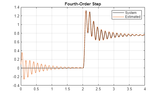
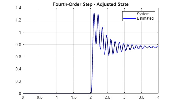
The plot shows two issues with the fit. First, the initial state of the network is not stationary, which results in transient behavior at the start of the signal. Second, the prediction of the network has a slight offset.
Initialize Network and Adjust Fit
To initialize the network state to the correct initial condition, you must update the network state to correspond to the state of the system at the start of the test signal.
You can adjust the initial state of the network by comparing the estimated response of the system at the initial condition to the actual response of the system. Use the difference between the estimation of the initial state by the network and the actual response of the initial state to correct for the offset in the system estimation.
Set Network Initial State
As the network performs estimation using a step input from 0 to 1, the states of the LSTM network (cell and hidden states of the LSTM layers) drift toward the correct initial condition. To visualize this, extract the cell and hidden state of the network at every time step using the predictAndUpdateState function.
Use only the cell and hidden state values prior to the step, which occurs at 2 seconds. Define a time marker for 2 seconds, and extract the values up to this marker.
stepMarker = time <= 2;
yhat = zeros(sum(stepMarker),1);
hiddenState = zeros(sum(stepMarker),200); % 200 LSTM units
cellState = zeros(sum(stepMarker),200);
for ntime = 1:sum(stepMarker)
    [fourthOrderNet,yhat(ntime)] = predictAndUpdateState(fourthOrderNet,stepSignal(ntime)');
    hiddenState(ntime,:) = fourthOrderNet.Layers(2,1).HiddenState;
    cellState(ntime,:) = fourthOrderNet.Layers(2,1).CellState;
end
Next, plot the hidden and cell states over the period before the step and confirm that they converge to fixed values.
figure
subplot(2,1,1)
plot(time(1:200),hiddenState(1:200,:))
grid on
axis tight
title('Hidden State')
subplot(2,1,2)
plot(time(1:200),cellState(1:200,:))
grid on
axis tight
title('Cell State')
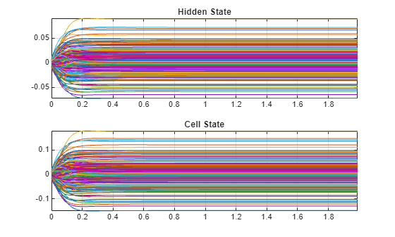
To initialize the network state for a zero input signal, choose an input signal of zero and choose the duration so that the signal is long enough for the networks to reach steady state.
initializationSignalDuration = 10; % In seconds
initializationValue = 0;
initializationSignal = initializationValue*ones(1,initializationSignalDuration*fs);

fourthOrderNet = predictAndUpdateState(fourthOrderNet,initializationSignal);
Verify that the initial condition is zero or close to zero.
figure
zeroMapping = predict(fourthOrderNet,initializationSignal);
plot(zeroMapping)
axis tight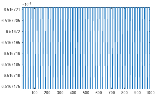
Now that the network is correctly initialized, use the network to predict the step response again and plot the results. The initial disturbance is gone.
fourthOrderMixedNetStep = predict(fourthOrderNet,stepSignal);

figure
title('Step response estimation')
plot(time,systemResponse,'k', ...
    time,fourthOrderMixedNetStep,'b')
grid on
legend('System','Estimated')
title('Fourth-Order Step - Adjusted State')
Adjust Network Offset
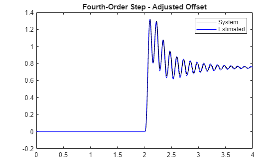
Even after you set the network initial state to compensate for the initial condition of the test signal, a small offset is still visible in the predicted response. This is because of the incorrect bias term that the LSTM network learned during training. You can fix the offset by using the same initialization signal that was used for updating the network states. The initialization signal is expected to map the network to zero. The offset between zero and the network estimation is the error in the bias term learned by the network. Summing the bias term calculated at each layer comes close to the bias detected in the response. Adjusting for the network bias term at the network output, however, is easier than adjusting the individual bias terms in each layer of the network.
bias = mean(predict(fourthOrderNet,initializationSignal));
fourthOrderMixedNetStep = fourthOrderMixedNetStep-bias;

figure
title('Step response estimation')
plot(time,systemResponse,'k',time,fourthOrderMixedNetStep,'b-')
legend('System','Estimated')
title('Fourth-Order Step - Adjusted Offset')
Move Outside of Training Range
All the signals used to train the network had a maximum amplitude of 1 and the step function had an amplitude of 0.1. Now, investigate the behavior of the network outside of these ranges.
Time Shift
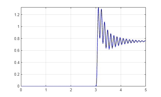
Introduce a time shift by adjusting the time of the step. Set the time of the step to 3 seconds, 1 second longer than in the training set. Plot the resulting network output and note that the output is correctly delayed by 1 second.
stepTime = 3; % In seconds
stepAmplitude = 0.1;
stepDuration = 5; % In seconds
[stepSignal,systemResponse,time] = generateStepResponse(fourthOrderMdl,stepTime,stepAmplitude,stepDuration);

fourthOrderMixedNetStep = predict(fourthOrderNet,stepSignal);
bias = fourthOrderMixedNetStep(1) - initializationValue;
fourthOrderMixedNetStep = fourthOrderMixedNetStep-bias;

figure
plot(time,systemResponse,'k', time,fourthOrderMixedNetStep,'b')
grid on
axis tight
Amplitude Shift
Next, increase the amplitude of the step function to investigate the network behavior as the system inputs move outside of the range of the training data. To measure the drift outside of the training data range, you can measure the probability density function of the amplitudes in the Gaussian noise signal. Visualize the amplitudes in a histogram.
figure
histogram(urgs,'Normalization','pdf')
grid on
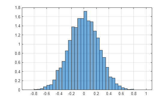
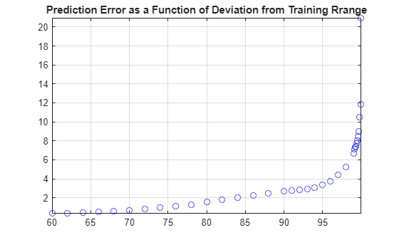
Set the amplitude of the step function according to the percentile of the distribution. Plot the error rate as a function of the percentile.
pValues = [60:2:98, 90:1:98, 99:0.1:99.9 99.99];
stepAmps = prctile(urgs,pValues); % Amplitudes
stepTime = 3; % In seconds
stepDuration = 5; % In seconds

stepMSE = zeros(length(stepAmps),1);
fourthOrderMixedNetStep = cell(length(stepAmps),1);
steps = cell(length(stepAmps),1);

for nAmps = 1:length(stepAmps)
    % Fourth-order mixed
    [stepSignal,systemResponse,time] = generateStepResponse(fourthOrderMdl,stepTime,stepAmps(nAmps),stepDuration);

    fourthOrderMixedNetStep{nAmps} = predict(fourthOrderNet,stepSignal);
    bias = fourthOrderMixedNetStep{nAmps}(1) - initializationValue;
    fourthOrderMixedNetStep{nAmps} = fourthOrderMixedNetStep{nAmps}-bias;

    stepMSE(nAmps) = sqrt(sum((systemResponse-fourthOrderMixedNetStep{nAmps}).^2));
    steps{nAmps,1} = systemResponse;
end

figure
plot(pValues,stepMSE,'bo')
title('Prediction Error as a Function of Deviation from Training Rrange')
grid on
axis tight
subplot(2,1,1)
plot(time,steps{1},'k', time,fourthOrderMixedNetStep{1},'b')
grid on
axis tight
title('Best Performance')
xlabel('time')
ylabel('System Response')
subplot(2,1,2)
plot(time,steps{end},'k', time,fourthOrderMixedNetStep{end},'b')
grid on
axis tight
title('Worst Performance')
xlabel('time')
ylabel('System Response')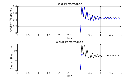
As the amplitude of the step response moves outside of the range of the training set, the LSTM attempts to estimate the average value of the response.
These results show the importance of using training data that is in the same range as the data that will be used for prediction. Otherwise, prediction results are unreliable.
Change System Bandwidth
Investigate the effect of the system bandwidth on the number of hidden units selected for the LSTM network by modeling the fourth-order mixed-dynamics transfer function with four different networks:
Small network with 5 hidden units and a single LSTM layer
Medium network with 10 hidden units and a single LSTM layer
Full network with 100 hidden units and a single LSTM layer
Deep network with 2 LSTM layers (each with 100 hidden units)
Load the trained networks.
load('variousHiddenUnitNets.mat')Generate a step signal.
stepTime = 2; % In seconds
stepAmplitude = 0.1;
stepDuration = 4; % In seconds

% Construct step signal.
time = (0:1/fs:stepDuration)';

stepSignal = [zeros(sum(time<=stepTime),1);stepAmplitude*ones(sum(time>stepTime),1)];
systemResponse = lsim(fourthOrderMdl,stepSignal,time);

% Transpose input and output signal for network inputs.
stepSignal = stepSignal';
systemResponse = systemResponse';
Estimate the system response using the various trained networks.
smallNetStep = predict(smallNet,stepSignal)-smallNetZeroMapping(end);
medNetStep = predict(medNet,stepSignal)-medNetZeroMapping(end);
fullnetStep = predict(fullNet,stepSignal) - fullNetZeroMapping(end);
doubleNetStep = predict(doubleNet,stepSignal) - doubleNetZeroMapping(end);
Plot the estimated response.
figure
title('Step response estimation')
plot(time,systemResponse,'k', ...
    time,doubleNetStep,'g', ...
    time,fullnetStep,'r', ...
    time,medNetStep,'c', ...
    time,smallNetStep,'b')
grid on
legend({'System','Double Net','Full Net','Med Net','Small Net'},'Location','northwest')
title('Fourth-Order Step')
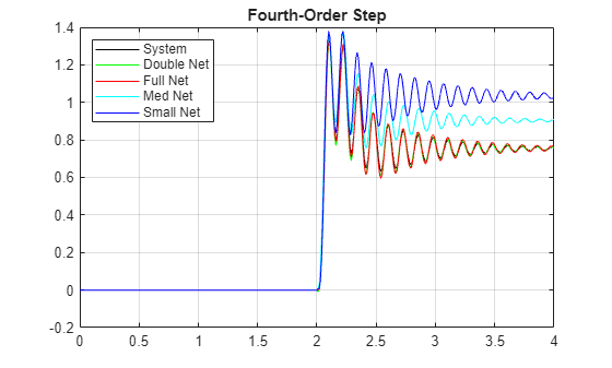
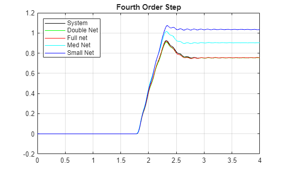
Note all the networks capture the high frequency dynamics in the response well. However, plot a moving average of the responses in order to compare the slow varying dynamics of the system. The ability of the LSTM to capture the longer term dynamics (lower frequency dynamics) of the linear system is directly related to the dynamics of the system and the number of hidden units in the LSTM. The number of layers in the LSTM is not directly related to the long-term behavior but rather adds flexibility to adjust the estimation from the first layer.
figure
title('Slow dynamics component')
plot(time,movmean(systemResponse,50),'k')
hold on
plot(time,movmean(doubleNetStep,50),'g')
plot(time,movmean(fullnetStep,50),'r')
plot(time,movmean(medNetStep,50),'c')
plot(time,movmean(smallNetStep,50),'b')
grid on
legend('System','Double Net','Full net','Med Net','Small Net','Location','northwest')
title('Fourth Order Step')
Add Noise to Measured System Response
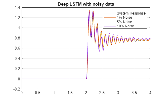
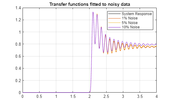
Add random noise to the system output to explore the effect of noise on the LSTM performance. To this end, add white noise with levels of 1%, 5%, and 10% to the measured system responses. Use the noisy data to train the LSTM network. With the same noisy data sets, estimate linear models by using tfest. Simulate these models and use the simulated responses as the baseline for a performance comparison.
Use the same step function as before:
stepTime = 2; % In seconds
stepAmplitude = 0.1;
stepDuration = 4; % In seconds

[stepSignal,systemResponse,time] = generateStepResponse(fourthOrderMdl,stepTime,stepAmplitude,stepDuration);
Load the trained networks and estimate the system response.
load('noisyDataNetworks.mat')
netNoise1Step = predictAndAdjust(netNoise1,stepSignal,initializationSignal,initializationValue);
netNoise5Step = predictAndAdjust(netNoise5,stepSignal,initializationSignal,initializationValue);
netNoise10Step = predictAndAdjust(netNoise10,stepSignal,initializationSignal,initializationValue);
A transfer function estimator (tfest) is used to estimate the function at the above noise levels to compare the resilience of the networks to noise (see the accompanying noiseLevelModels.m for more details).
load('noisyDataTFs.mat')
tfStepNoise1 = lsim(tfNoise1,stepSignal,time);
tfStepNoise5 = lsim(tfNoise5,stepSignal,time);
tfStepNoise10 = lsim(tfNoise10,stepSignal,time);
Plot the generated responses.
figure
plot(time,systemResponse,'k', ...
    time,netNoise1Step, ...
    time,netNoise5Step, ...
    time,netNoise10Step)
grid on
legend('System Response','1% Noise','5% Noise','10% Noise')
title('Deep LSTM with noisy data')
Now, plot the estimated transfer functions.
figure
plot(time,systemResponse,'k', ...
    time,tfStepNoise1, ...
    time,tfStepNoise5, ...
    time,tfStepNoise10)
grid on
legend('System Response','1% Noise','5% Noise','10% Noise')
title('Transfer functions fitted to noisy data')
Calculate the mean squared error to better assess the performance of the different models at different noise levels.
msefun = @(y,yhat) mean(sqrt((y-yhat).^2)/length(y));

% LSTM errors
lstmMSE(1,:) = msefun(systemResponse,netNoise1Step);
lstmMSE(2,:) = msefun(systemResponse,netNoise5Step);
lstmMSE(3,:) = msefun(systemResponse,netNoise10Step);

% Transfer function errors
tfMSE(1,:) = msefun(systemResponse,tfStepNoise1');
tfMSE(2,:) = msefun(systemResponse,tfStepNoise5');
tfMSE(3,:) = msefun(systemResponse,tfStepNoise10');

mseTbl = array2table([lstmMSE tfMSE],'VariableNames',{'LSTMMSE','TFMSE'})
mseTbl = 3×2 table
    1.0115e-05    8.8621e-07
    2.5577e-05    9.9064e-06
    5.1791e-05    3.6831e-05
Noise has a similar effect on both the LSTM and transfer-function estimation results.
Helper Functions
function [stepSignal,systemResponse,time] = generateStepResponse(model,stepTime,stepAmp,signalDuration)
%Generates a step response for the given model.
%

%Check model type
modelType = class(model);
if nargin < 2
    stepTime = 1;
end

if nargin < 3
    stepAmp = 1;
end

if nargin < 4
    signalDuration = 10;
end

% Construct step signal
if model.Ts == 0
    Ts = 1e-2;
    time = (0:Ts:signalDuration)';
else
    time = (0:model.Ts:signalDuration)';
end
stepSignal = [zeros(sum(time<=stepTime),1);stepAmp*ones(sum(time>stepTime),1)];
switch modelType
    case {'tf', 'zpk'}
        systemResponse = lsim(model,stepSignal,time);
    case 'idpoly'
        systemResponse = sim(model,stepSignal,time);
    otherwise
        error('Model passed is not supported')
end

stepSignal = stepSignal';
systemResponse = systemResponse';
end

