Compute Statistics for Large Images

Step 1: Create a Truecolor Composite

Using blockproc, read the data from rio.lan, a file containing Landsat thematic mapper imagery in the Erdas LAN file format. blockproc has built-in support for reading TIFF and JPEG2000 files only. To read other types of files you must write an Image Adapter class to support I/O for your particular file format. This example uses a pre-built Image Adapter class, the LanAdapter, which supports reading LAN files. For more information on writing Image Adapter classes, see Perform Block Processing on Image Files in Unsupported Formats.

The Erdas LAN format contains the visible red, green, and blue spectrum in bands 3, 2, and 1, respectively. Use blockproc to extract the visible bands into an RGB image.

Create the LanAdapter object associated with rio.lan.

input_adapter = LanAdapter("rio.lan");

Select the visible R, G, and B bands.

input_adapter.SelectedBands = [3 2 1];

Create a simple block function that returns the block data unchanged.

identityFcn = @(block_struct) block_struct.data;

Create the initial truecolor image.

truecolor = blockproc(input_adapter,[100 100],identityFcn);

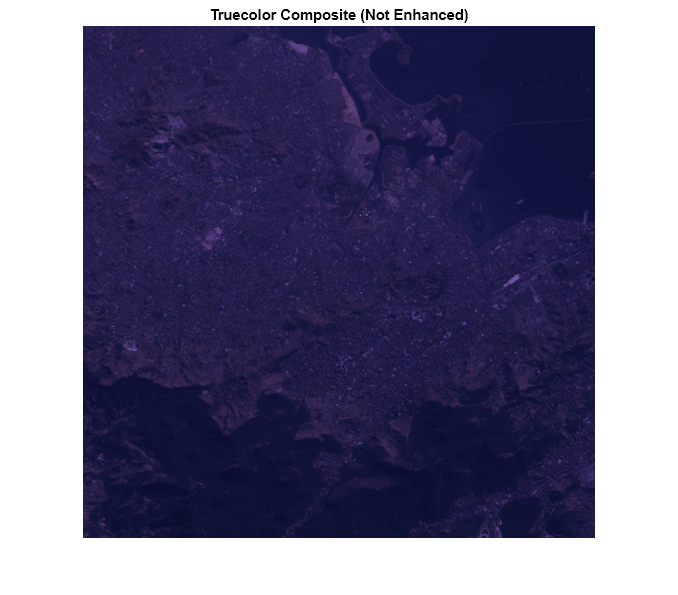
Display the results before enhancement.

imshow(truecolor)
title("Truecolor Composite (Not Enhanced)")

The resulting truecolor image is similar to that of paris.lan in the Enhance Multispectral Color Composite Images example. The RGB image appears dull, with little contrast.

Step 2: Enhance the Image - First Attempt

First, try to stretch the data across the dynamic range using blockproc. This first attempt simply defines a new function handle that calls stretchlim and imadjust on each block of data individually.

adjustFcn = @(block_struct) imadjust(block_struct.data, ...
    stretchlim(block_struct.data));
truecolor_enhanced = blockproc(input_adapter,[100 100],adjustFcn);

imshow(truecolor_enhanced)
title("Truecolor Composite with Blockwise Contrast Stretch")

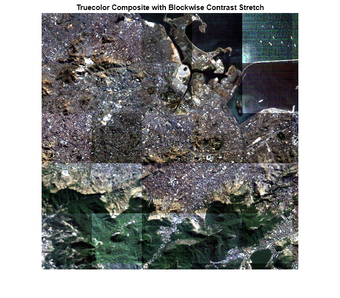
You can see immediately that the results are incorrect. The problem is that the stretchlim function computes the histogram on the input image and uses this information to compute the stretch limits. Since each block is adjusted in isolation from its neighbors, each block is computing different limits from its local histogram.

Step 3: Examine the Histogram Accumulator Class

To examine the distribution of data across the dynamic range of the image, you can compute the histogram for each of the three visible bands.

When working with sufficiently large images, you cannot simply call imhist to create an image histogram. One way to incrementally build the histogram is to use blockproc with a class that will sum the histograms of each block as you move over the image.

Examine the HistogramAccumulator class.

type HistogramAccumulator

% HistogramAccumulator Accumulate incremental histogram.
%   HistogramAccumulator is a class that incrementally builds up a
%   histogram for an image.  This class is appropriate for use with 8-bit
%   or 16-bit integer images and is for educational purposes ONLY.

%   Copyright 2009 The MathWorks, Inc.

classdef HistogramAccumulator < handle
   
    properties
        Histogram
        Range
    end
    
    methods
        
        function obj = HistogramAccumulator()
            obj.Range = [];
            obj.Histogram = [];
        end
        
        function addToHistogram(obj,new_data)
            if isempty(obj.Histogram)
                obj.Range = double(0:intmax(class(new_data)));
                obj.Histogram = hist(double(new_data(:)),obj.Range);
            else
                new_hist = hist(double(new_data(:)),obj.Range);
                obj.Histogram = obj.Histogram + new_hist;
            end
        end
    end
end

The class is a simple wrapper around the hist function, allowing you to add data to a histogram incrementally. It is not specific to blockproc. Observe the following simple use of the HistogramAccumulator class.

Create the HistogramAccumulator object.

hist_obj = HistogramAccumulator;

Split a sample image into 2 halves.

full_image = imread("liftingbody.png");
top_half = full_image(1:256,:);
bottom_half = full_image(257:end,:);

Compute the histogram incrementally.

addToHistogram(hist_obj,top_half);
addToHistogram(hist_obj,bottom_half);
computed_histogram = hist_obj.Histogram;

Compare against the results of the imhist function.

normal_histogram = imhist(full_image);

Examine the results. The histograms are numerically identical.

figure
subplot(1,2,1)
stem(computed_histogram,"Marker","none")
title("Incrementally Computed Histogram")
subplot(1,2,2)
stem(normal_histogram',"Marker","none")
title("imhist Histogram")

Step 4: Use the HistogramAccumulator Class with blockproc

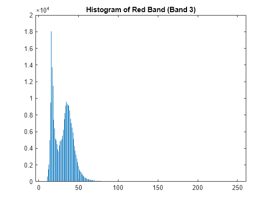
Use the HistogramAccumulator class with blockproc to build the histogram of the red band of data in rio.lan. You can define a function handle for blockproc that will invoke the addToHistogram method on each block of data. By viewing this histogram, you can see that the data is concentrated within a small part of the available dynamic range. The other visible bands have similar distributions. This is one reason why the original truecolor composite appears dull.

Create the HistogramAccumulator object.

hist_obj = HistogramAccumulator;

Set up blockproc function handle

addToHistFcn = @(block_struct) addToHistogram(hist_obj, block_struct.data);

Compute the histogram of the red channel. Notice that the addToHistFcn function handle does not generate any output. Since the function handle passed to blockproc does not return anything, blockproc will not return anything either.

input_adapter.SelectedBands = 3;
blockproc(input_adapter,[100 100],addToHistFcn);
red_hist = hist_obj.Histogram;

Display the results.

figure
stem(red_hist,"Marker","none")
title("Histogram of Red Band (Band 3)")

Step 5: Enhance the Truecolor Composite with a Contrast Stretch

You can now perform a proper contrast stretch on the image. For conventional, in-memory workflows, you can simply use the stretchlim function to compute the arguments to imadjust (like the example Enhance Multispectral Color Composite Images). When working with large images, as we have seen, stretchlim is not easily adapted for use with blockproc since it relies on the full image histogram.

Once you have computed the image histograms for each of the visible bands, compute the proper arguments to imadjust by hand (similar to how stretchlim does).

First compute the histograms for the green and blue bands.

hist_obj = HistogramAccumulator;
addToHistFcn = @(block_struct) addToHistogram(hist_obj,block_struct.data);
input_adapter.SelectedBands = 2;
blockproc(input_adapter,[100 100],addToHistFcn);
green_hist = hist_obj.Histogram;

hist_obj = HistogramAccumulator;
addToHistFcn = @(block_struct) addToHistogram(hist_obj,block_struct.data);
input_adapter.SelectedBands = 1;
blockproc(input_adapter,[100 100],addToHistFcn);
blue_hist = hist_obj.Histogram;

Compute the CDF of each histogram.

computeCDF = @(histogram) cumsum(histogram) / sum(histogram);
findLowerLimit = @(cdf) find(cdf > 0.01, 1, "first");
findUpperLimit = @(cdf) find(cdf >= 0.99, 1, "first");

red_cdf = computeCDF(red_hist);
red_limits(1) = findLowerLimit(red_cdf);
red_limits(2) = findUpperLimit(red_cdf);

green_cdf = computeCDF(green_hist);
green_limits(1) = findLowerLimit(green_cdf);
green_limits(2) = findUpperLimit(green_cdf);

blue_cdf = computeCDF(blue_hist);
blue_limits(1) = findLowerLimit(blue_cdf);
blue_limits(2) = findUpperLimit(blue_cdf);

Prepare the arguments for the imadjust function.

rgb_limits = [red_limits' green_limits' blue_limits'];

Scale to the range [0, 1].

rgb_limits = (rgb_limits - 1) / (255);

Create a new adjustFcn that applies the global stretch limits and use blockproc to adjust the truecolor image.

adjustFcn = @(block_struct) imadjust(block_struct.data,rgb_limits);

Select the full RGB data.

input_adapter.SelectedBands = [3 2 1];
truecolor_enhanced = blockproc(input_adapter,[100 100],adjustFcn);

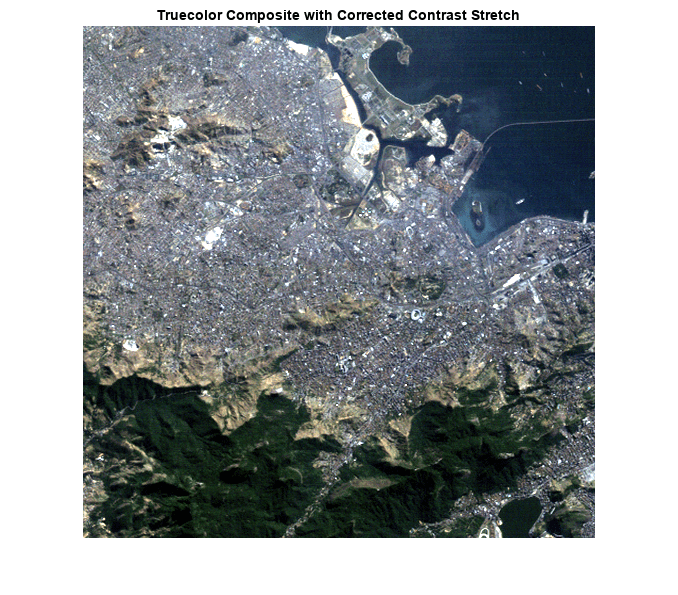
Display the result. The resulting image is much improved, with the data covering more of the dynamic range. By using blockproc you avoid loading the whole image into memory.

imshow(truecolor_enhanced)
title("Truecolor Composite with Corrected Contrast Stretch")