Adapt Blind Deconvolution for Various Image Distortions
Use the deconvblind function to deblur an image
using the blind deconvolution algorithm. The algorithm maximizes the likelihood that the
resulting image, when convolved with the resulting PSF, is an instance of the blurred
image, assuming Poisson noise statistics. The blind deconvolution algorithm can be used
effectively when no information about the distortion (blurring and noise) is known. The
deconvblind function restores the image and the PSF
simultaneously, using an iterative process similar to the accelerated, damped
Lucy-Richardson algorithm.
The deconvblind function, just like the
deconvlucy function, implements several adaptations to the
original Lucy-Richardson maximum likelihood algorithm that address complex image
restoration tasks. Using these adaptations, you can
Reduce the effect of noise on the restoration
Account for nonuniform image quality (such as bad pixels)
Handle camera read-out noise
For more information about these adaptations, see Adapt the Lucy-Richardson Deconvolution for Various Image Distortions. The
deconvblind function also supports PSF constraints that you can
provide through a user-specified function.
Deblur Images Using Blind Deconvolution
This example shows how to deblur an image using blind deconvolution. The example illustrates the iterative nature of this operation, making two passes at deblurring the image using optional parameters.
Read an image into the workspace and display it.
I = imread("cameraman.tif");
imshow(I)
title("Original Image")

Create a point spread function (PSF). A PSF describes the degree to which an optical system blurs (spreads) a point of light.
PSF = fspecial("motion",13,45);
figure
imshow(PSF,[],InitialMagnification="fit")
title("Original PSF")

Create a simulated blur in the image, using the PSF, and display the blurred image.
Blurred = imfilter(I,PSF,"circ","conv");
imshow(Blurred)
title("Blurred Image")
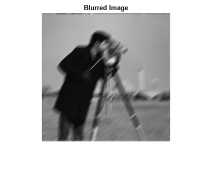
Deblur the image using the deconvblind function. You must make an initial guess at the PSF. To determine the size of the PSF, examine the blurred image and measure the width of a blur (in pixels) around an obviously sharp object. Because the size of the PSF is more important than the values it contains, you can typically specify an array of 1"s as the initial PSF.
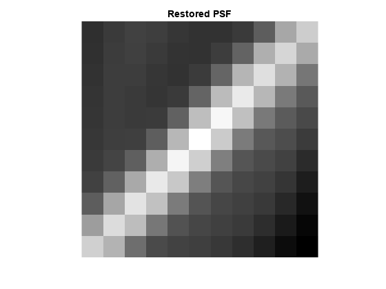
In this initial restoration, deconvblind was able to deblur the image to a great extent. Note, however, the ringing around the sharp intensity contrast areas in the restored image. (The example eliminated edge-related ringing by using the "circular" option with imfilter when creating the simulated blurred image.) To achieve a more satisfactory result, rerun the operation, experimenting with PSFs of different sizes. The restored PSF returned by each deconvolution can also provide valuable hints at the optimal PSF size.
initPSF = ones(size(PSF));
[J,P] = deconvblind(Blurred,initPSF,30);
imshow(J)
title("Restored Image")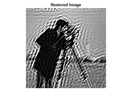
imshow(P,[],InitialMagnification="fit")
title("Restored PSF")
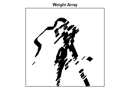
One way to improve the result is to create a weight array to exclude areas of high contrast from the deblurring operation. This can reduce contrast-related ringing in the result.
To create a weight array, create an array the same size as the image, and assign the value 0 to the pixels in the array that correspond to pixels in the original image that you want to exclude from processing. The example uses a combination of edge detection and morphological processing to detect high-contrast areas in the image. Because the blur in the image is linear, the example dilates the image twice. To exclude the image boundary pixels (a high-contrast area) from processing, the example uses padarray to assign the value 0 to all border pixels.
WEIGHT = edge(I,"sobel",.28);
se1 = strel("disk",1);
se2 = strel("line",13,45);
WEIGHT = ~imdilate(WEIGHT,[se1 se2]);
WEIGHT = padarray(WEIGHT(2:end-1,2:end-1),[1 1]);
imshow(WEIGHT)
title("Weight Array")
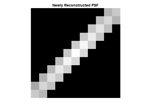
Refine the guess at the PSF. The reconstructed PSF returned by the first pass at deconvolution, P, shows a clear linearity. For this second pass, the example uses a new PSF which is the same as the returned PSF but with the small amplitude pixels set to 0.
P1 = P;
P1(P1<0.01) = 0;
Run the deconvolution again, this time specifying the weight array and the modified PSF. Note how the restored image has much less ringing around the sharp intensity areas than the result of the first pass.
[J2,P2] = deconvblind(Blurred,P1,50,[],double(WEIGHT));
imshow(J2)
title("Newly Deblurred Image");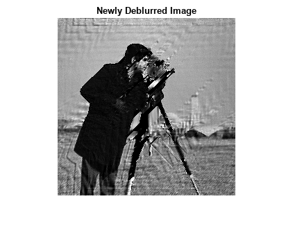
imshow(P2,[],InitialMagnification="fit")
title("Newly Reconstructed PSF")
Refining the Result
The deconvblind function, by default, performs multiple
iterations of the deblurring process. You can stop the processing after a certain
number of iterations to check the result, and then restart the iterations from the
point where processing stopped. To use this feature, you must pass in both the
blurred image and the PSF as cell arrays, for example, {Blurred}
and {INITPSF}.
The deconvblind function returns the output image and the
restored PSF as cell arrays. The output image cell array contains these four
elements:
Element | Description |
|---|---|
| Original input image |
| Image produced by the last iteration |
| Image produced by the next to last iteration |
| Internal information used by |
The PSF output cell array contains similar elements.