Granulometry of Snowflakes
This example shows how to calculate the size distribution of snowflakes in an image by using granulometry. Granulometry determines the size distribution of objects in an image without explicitly segmenting (detecting) each object first.
Read Image
Read in the snowflakes.png image, which is a photograph of snowflakes.
I = imread("snowflakes.png");
imshow(I)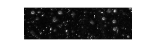
Enhance Contrast
Your first step is to maximize the intensity contrast in the image. You can do this using the adapthisteq function, which performs contrast-limited adaptive histogram equalization. Rescale the image intensity using the imadjust function so that it fills the data type's entire dynamic range.
claheI = adapthisteq(I,"NumTiles",[10 10]);
claheI = imadjust(claheI);
imshow(claheI)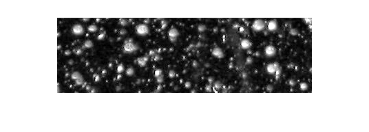
Determine Volume Under Image Surface in Enhanced Image
Granulometry is analogous to sifting stones through screens of increasing size and collecting what remains after each pass. Granulometry applies a series of morphological openings of increasing size, and the sum of image pixel values is computed after each opening. For grayscale images, this sum corresponds to the volume under the surface whose height is determined by the pixel intensity values. The volume is reduced after each opening as larger objects are eliminated by increasingly large structuring elements.
Optionally, you can plot the intensity surface of the snowflake image to conceptualize the surface volume. Adjust the vertical aspect ratio to make the whole surface visible. Surface peaks correspond to bright areas in the original 2-D image.
figure
surf(claheI, EdgeColor="none")
colormap("gray")
title("Snowflakes Pixel Intensity Surface")
daspect([1 1 15]);
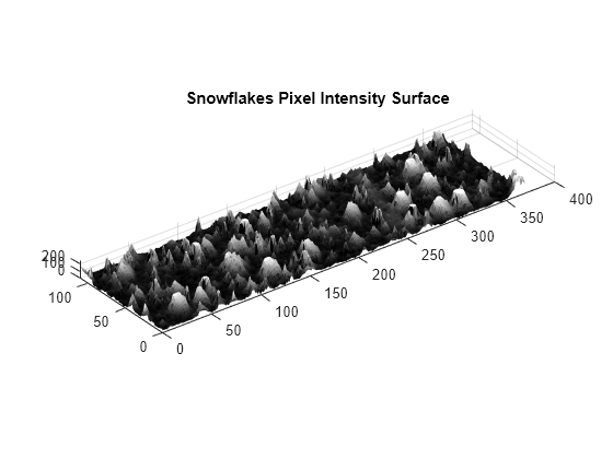
Choose a counter limit so that the intensity surface volume goes to zero as you increase the size of your structuring element. For display purposes, leave the first entry in the surface area array empty.
radius_range = 0:22;
intensity_volume = zeros(size(radius_range));
for counter = radius_range
    remain = imopen(claheI, strel("disk", counter));
    intensity_volume(counter + 1) = sum(remain(:));
end
figure
plot(intensity_volume, "m - *")
grid on
title("Sum of Pixel Values in Opened Image Versus Radius")
xlabel("Radius of Opening Structuring Element (pixels)")
ylabel("Sum of Pixel Values in Opened Image (intensity)")
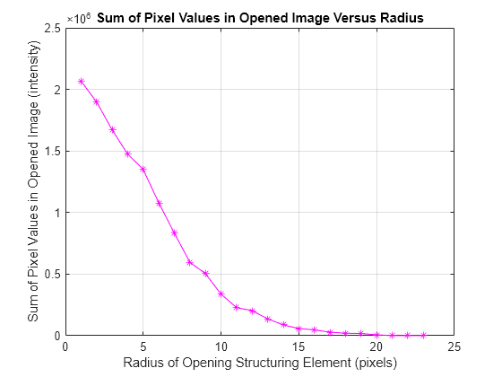
Estimate Derivative of Distribution
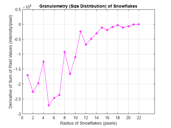
A significant drop in intensity surface volume between two consecutive openings indicates that the image contains objects of comparable size to the smaller opening. This is equivalent to the derivative of the intensity surface volume with respect to radius, which contains the size distribution of the snowflakes in the image. Estimate the derivative by using the diff function.
intensity_volume_prime = diff(intensity_volume);
figure
plot(intensity_volume_prime, "m - *")
grid on
title("Granulometry (Size Distribution) of Snowflakes")
ax = gca;
ax.XTick = [0 2 4 6 8 10 12 14 16 18 20 22];
xlabel("Radius of Snowflakes (pixels)")
ylabel("Derivative of Sum of Pixel Values (intensity/pixel)")
Emphasize Snowflakes Having a Particular Radius
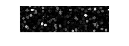
Notice the minima and the radii where they occur in the graph. The minima tell you that snowflakes in the image have those radii. The more negative the minimum point, the higher the snowflakes' cumulative intensity at that radius. For example, the most negative minimum point occurs at the 5 pixel radius mark. You can emphasize the snowflakes having a 5 pixel radius with the following steps.
open5 = imopen(claheI,strel("disk",5));
open6 = imopen(claheI,strel("disk",6));
rad5 = open5 - open6;
imshow(rad5,[])
See Also
adapthisteq | imadjust | imopen | strel