Reduce the Number of Colors in an Image

To reduce the number of colors in a truecolor image, use the rgb2ind function. This function converts a truecolor image to an indexed image, reducing the number of colors in the process. rgb2ind provides the following methods for approximating the colors in the original image:

To reduce the number of colors in an indexed image, use the imapprox function. For more information, see Reduce Colors of Indexed Image Using imapprox.

The quality of the resulting image depends on the approximation method you use, the range of colors in the input image, and whether or not you use dithering. See Reduce Colors Using Dithering for a description of dithering and how to enable or disable it. Note that different approximation methods work better for different images.

Reduce Colors of Truecolor Image Using Quantization

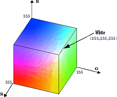
The rgb2ind function uses quantization as part of its color reduction algorithm. Quantization involves dividing the RGB color cube into a number of smaller boxes, and then mapping all colors that fall within each box to the color value at the center of that box. The RGB color cube is a three-dimensional array of all of the colors that are defined for a particular data type.

The color cubes for uint8, uint16, and double images all have the same range of colors. In other words, the brightest red in a uint8 RGB image appears the same as the brightest red in a double RGB image. The difference is that the double RGB color cube has many more shades of red (and many more shades of all colors). The following figure shows an RGB color cube for a uint8 image.

RGB Color Cube for uint8 Images

RGB color cube in 3-D space with axes R, G, and B. The color white is the opposite corner from the origin, at coordinate (255, 255, 255).

rgb2ind supports two quantization methods:

In uniform quantization, the color cube is divided into equal-sized boxes (smaller cubes).
In minimum variance quantization, the color cube is cut up into boxes (not necessarily cubes) of different sizes. The sizes of the boxes depend on how the colors are distributed in the image.

Uniform Quantization

To perform uniform quantization, call rgb2ind and specify a tolerance. The tolerance determines the size of the cube-shaped boxes into which the RGB color cube is divided. The allowable range for a tolerance setting is [0,1]. For example, if you specify a tolerance of 0.1, then the edges of the boxes are one-tenth the length of the RGB color cube and the maximum total number of boxes is:

n = (floor(1/tol)+1)^3

The commands below perform uniform quantization with a tolerance of 0.1.

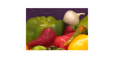
RGB = imread("peppers.png");
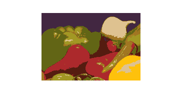
[x,map] = rgb2ind(RGB, 0.1);

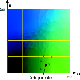
The following figure illustrates uniform quantization of a uint8 image with a tolerance of 0.25. For clarity, the figure shows a two-dimensional slice (or color plane) from the color cube where red=0 and green and blue range from 0 to 255. The actual pixel values are denoted by the centers of the x markers.

Uniform Quantization on a Slice of the RGB Color Cube

Slice of the RGB color cube in the G-B plane, divided into 16 square boxes of uniform size. The RGB coordinates of five pixels appear with an x symbol and all pixels happen to be located within a single box of the quantized plane for this sample image.

After the color cube has been divided, all empty boxes are thrown out. Therefore, only one of the boxes is used to produce a color for the colormap. As shown earlier, the maximum length of a colormap created by uniform quantization can be predicted, but the colormap can be smaller than the prediction because rgb2ind removes any colors that do not appear in the input image.

Minimum Variance Quantization

To perform minimum variance quantization, call rgb2ind and specify the maximum number of colors in the output image's colormap. The number you specify determines the number of boxes into which the RGB color cube is divided. These commands use minimum variance quantization to create an indexed image with 185 colors.

RGB = imread("peppers.png");
[X,map] = rgb2ind(RGB,185);

Minimum variance quantization works by associating pixels into groups based on the variance between their pixel values. For example, a set of blue pixels might be grouped together because they have a small variance from the center pixel of the group.

In minimum variance quantization, the boxes that divide the color cube vary in size, and do not necessarily fill the color cube. If some areas of the color cube do not have pixels, there are no boxes in these areas.

While you set the number of boxes, n, to be used by rgb2ind, the placement is determined by the algorithm as it analyzes the color data in your image. Once the image is divided into n optimally located boxes, the pixels within each box are mapped to the pixel value at the center of the box, as in uniform quantization.

The resulting colormap usually has the number of entries you specify. This is because the color cube is divided so that each region contains at least one color that appears in the input image. If the input image uses fewer colors than the number you specify, the output colormap will have fewer than n colors, and the output image will contain all of the colors of the input image.

The following figure shows the same two-dimensional slice of the color cube as shown in the preceding figure (demonstrating uniform quantization). Eleven boxes have been created using minimum variance quantization.

Minimum Variance Quantization on a Slice of the RGB Color Cube

Slice of the RGB color cube in the G-B plane, divided into 11 rectangular boxes of nonuniform size. The RGB coordinates of several pixels appear with an x symbol and the boxes surround clusters of pixels with similar coordinates.

For a given number of colors, minimum variance quantization produces better results than uniform quantization, because it takes into account the actual data. Minimum variance quantization allocates more of the colormap entries to colors that appear frequently in the input image. It allocates fewer entries to colors that appear infrequently. As a result, the accuracy of the colors is higher than with uniform quantization. For example, if the input image has many shades of green and few shades of red, there will be more greens than reds in the output colormap. Note that the computation for minimum variance quantization takes longer than that for uniform quantization.

Reduce Colors of Truecolor Image Using Colormap Mapping

If you specify a target colormap, rgb2ind uses colormap mapping instead of quantization. Colormap mapping finds the colors in the specified colormap that best match the colors in the RGB image. This method is useful if you need to create images that use a fixed colormap. For example, if you want to display multiple indexed images on an 8-bit display, you can avoid color problems by mapping them all to the same colormap. Colormap mapping produces a good approximation if the specified colormap has similar colors to those in the RGB image. If the colormap does not have similar colors to those in the RGB image, this method produces poor results.

This example illustrates mapping two images to the same colormap. The colormap used for the two images is created on the fly using the colorcube function, which creates an RGB colormap containing the number of colors that you specify. (colorcube always creates the same colormap for a given number of colors.) Because the colormap includes colors all throughout the RGB color cube, the output images can reasonably approximate the input images.

RGB1 = imread("autumn.tif");
RGB2 = imread("peppers.png");
X1 = rgb2ind(RGB1,colorcube(128));
X2 = rgb2ind(RGB2,colorcube(128));

Reduce Colors of Indexed Image Using `imapprox`

Use imapprox when you need to reduce the number of colors in an indexed image. imapprox is based on rgb2ind and uses the same approximation methods. Essentially, imapprox first calls ind2rgb to convert the image to RGB format, and then calls rgb2ind to return a new indexed image with fewer colors.

For example, these commands create a version of the trees image with 64 colors, rather than the original 128.

load trees
[Y,newcmap] = imapprox(X,map,64);
imshow(Y,newcmap)

Indexed images might cause problems if they have a large number of colors. In general, you should limit indexed images to 256 colors for the following reasons:

On systems with 8-bit display, indexed images with more than 256 colors need to be dithered or mapped and, therefore, might not display well.
On some platforms, colormaps cannot exceed 256 entries.
If an indexed image has more than 256 colors, MATLAB^® cannot store the image data in a uint8 array. Instead, MATLAB generally uses an array of data type double, which makes the storage size of the image much larger because each pixel uses 64 bits.
Most image file formats limit indexed images to 256 colors. If you write an indexed image with more than 256 colors (using imwrite) to a format that does not support more than 256 colors, you will receive an error.

Reduce Colors Using Dithering

Open Live Script

When you use rgb2ind or imapprox to reduce the number of colors in an image, the resulting image might look inferior to the original, because some of the colors are lost. rgb2ind and imapprox both perform dithering to increase the apparent number of colors in the output image. Dithering changes the colors of pixels in a neighborhood so that the average color in each neighborhood approximates the original RGB color.

For an example of how dithering works, consider an image that contains a number of dark orange pixels for which there is no exact match in the colormap. To create the appearance of this shade of orange, dithering selects a combination of colors from the colormap, that, taken together as a six-pixel group, approximate the desired shade of orange. From a distance, the pixels appear to be the correct shade, but if you look up close at the image, you can see a blend of other shades. To illustrate dithering, the following example loads a 24-bit truecolor image, and then uses rgb2ind to create an indexed image with just eight colors. The first example does not use dithering, the second does use dithering.

Read image and display it.

rgb = imread('onion.png'); 
imshow(rgb)

Figure contains an axes object. The hidden axes object contains an object of type image.

Create an indexed image with eight colors and without dithering.

[X_no_dither,map] = rgb2ind(rgb,8,'nodither');
imshow(X_no_dither,map)

Figure contains an axes object. The hidden axes object contains an object of type image.

Create an indexed image using eight colors with dithering. Notice that the dithered image has a larger number of apparent colors but is somewhat fuzzy-looking. The image produced without dithering has fewer apparent colors, but an improved spatial resolution when compared to the dithered image. One risk in doing color reduction without dithering is that the new image can contain false contours.

[X_dither,map] = rgb2ind(rgb,8,'dither');
imshow(X_dither,map)

Figure contains an axes object. The hidden axes object contains an object of type image.